[Avg. reading time: 0 minutes]
[Avg. reading time: 0 minutes]
Disclaimer


[Avg. reading time: 4 minutes]
Required Tools
System Setup
-
CLI
-
Python (3.11–3.13 recommended)
-
Python Dependency Manager (choose one)
-
Code Editor
-
VSCode Extension
-
Container Engine (choose one)
Free Cloud Services
| Tool | Purpose | Link |
|---|---|---|
| Redis | In-memory DB, caching | Redis Labs |
| GUI client | Redis Insight | |
| MongoDB | NoSQL Document DB | MongoDB Atlas |
| Neo4j | Graph DB for relationship data | Neo4j Console |
[Avg. reading time: 2 minutes]
Big Data Overview
- Introduction
- Job Opportunities
- What is Data?
- How does it help?
- Types of Data
- The Big V’s
- Trending Technologies
- Big Data Concerns
- Big Data Challenges
- Data Integration
- Scaling
- Cap Theorem
- Optimistic Concurrency
- Eventual Consistency
- Concurrent vs Parallel
- GPL
- DSL
- Big Data Tools
- NO Sql Databases
- What does Big Data learning means?
#introduction #bigdata #chapter1
[Avg. reading time: 2 minutes]
Understanding the Big Data Landscape
Expectation in this course
The first set of questions, which everyone is curious to know.
What is Big Data?
When does the data become Big Data?
Why collect so much Data?
How secure is Big Data?
How does it help?
Where can it be stored?
Which Tools are used to handle Big Data?
The second set of questions to get in deep.
What should I learn?
Does certification help?
Which technology is the best?
How many tools do I need to learn?
Apart from the top 50 corporations, do other companies use Big Data?
[Avg. reading time: 3 minutes]
Job Opportunities
| Role | On-Prem | Big Data Specific | Cloud |
|---|---|---|---|
| Database Developer | ✅ | ✅ | ✅ |
| Data Engineer | ✅ | ✅ | ✅ |
| Database Administrator | ✅ | ✅ | ✅ |
| Data Architect | ✅ | ✅ | ✅ |
| Database Security Eng. | ✅ | ✅ | ✅ |
| Database Manager | ✅ | ✅ | ✅ |
| Data Analyst | ✅ | ✅ | ✅ |
| Business Intelligence | ✅ | ✅ | ✅ |
Database Developer: Designs and writes efficient queries, procedures, and data models for structured databases.
Data Engineer: Builds and maintains scalable data pipelines and ETL processes for large-scale data movement and transformation.
Database Administrator (DBA): Manages and optimizes database systems, ensuring performance, security, and backups.
Data Architect: Defines high-level data strategy and architecture, ensuring alignment with business and technical needs.
Database Security Engineer: Implements and monitors security controls to protect data assets from unauthorized access and breaches.
Database Manager: Oversees database teams and operations, aligning database strategy with organizational goals.
Data Analyst: Interprets data using statistical tools to generate actionable insights for decision-makers.
Business Intelligence (BI) Developer: Creates dashboards, reports, and visualizations to help stakeholders understand data trends and KPIs.
All small to enterprise organizations use Big data to develop their business.
[Avg. reading time: 4 minutes]
What is Data?
Data is simply facts and figures.
When processed and contextualized, data becomes information.
Everything is data
What we say
Where we go
What we do
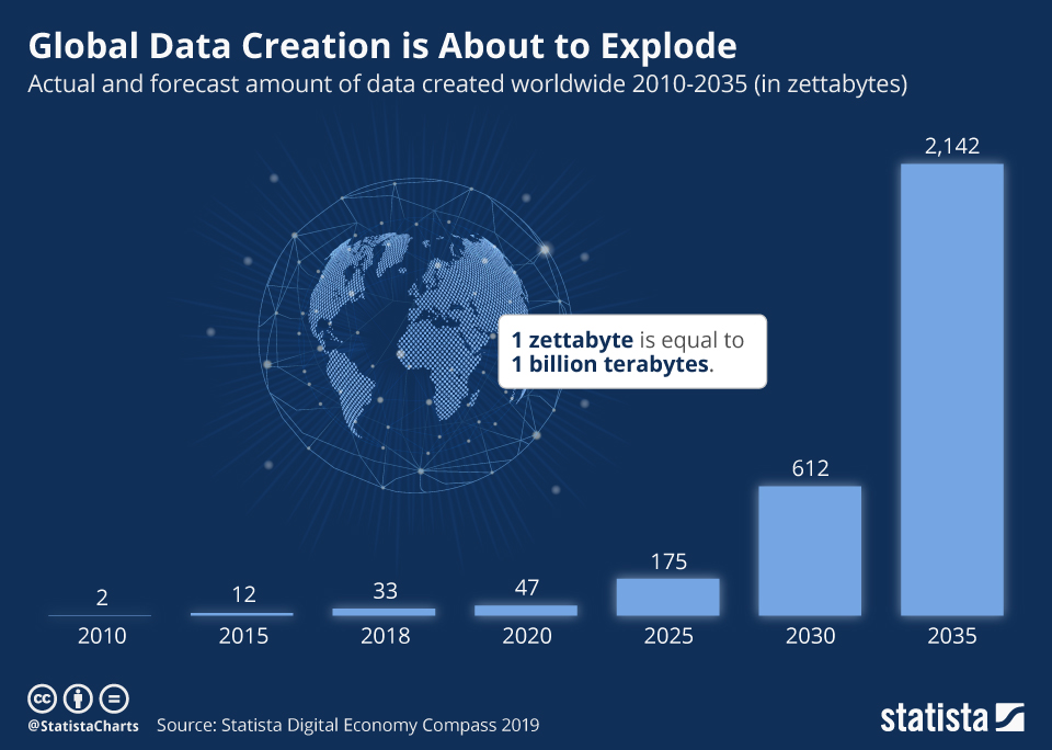
How to measure data?
byte        - 1 letter
1 Kilobyte  - 1024 B
1 Megabyte  - 1024 KB
1 Gigabyte  - 1024 MB
1 Terabyte  - 1024 GB
(1,099,511,627,776 Bytes)
1 Petabyte  - 1024 TB
1 Exabyte   - 1024 PB
1 Zettabyte - 1024 EB
1 Yottabyte - 1024 ZB
Examples of Traditional Data
- 🏦 Banking Records
- 🎓 Student Information
- 👩💼 Employee Profiles
- 🧾 Customer Details
- 💰 Sales Transactions
When Data becomes Big Data?
When data expands
- Banking: One bank branch vs. global consolidation (e.g., CitiBank)
- Education: One college vs. nationwide student data (e.g., US News)
- Media: Traditional news vs. user-generated content on Social Media
When data gets granular
- Monitoring CPU/Memory usage every second
- Cell phone location & usage logs
- IoT sensor telemetry (temperature, humidity, etc.)
- Social media posts, reactions, likes
- Live traffic data from vehicles and sensors
These fine-grained data points fuel powerful analytics and real-time insights.
Why Collect So Much Data?
- Storage is cheap and abundant
- Tech has advanced to process massive data efficiently
- Businesses use data to innovate, predict trends, and grow
#data #bigdata #traditionaldata
[Avg. reading time: 3 minutes]
How Big Data helps us
From raw blocks to building knowledge, Big Data drives global progress.
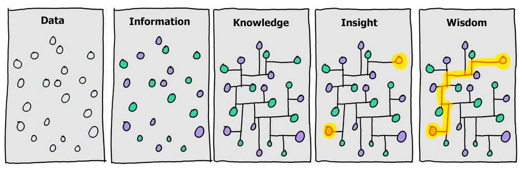
Stages
- Data → scattered observations
- Information → contextualized
- Knowledge → structured relationships
- Insight → patterns emerge
- Wisdom → actionable strategy
Raw Data to Analysis
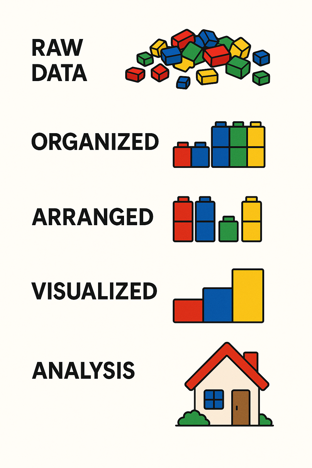
Stages
- Raw Data – Messy, unprocessed
- Organized – Grouped by category
- Arranged – Structured to show comparisons
- Visualized – Charts or graphs
- Analysis – Final understanding or solution
Big Data Applications: Changing the World
Here are some real-world domains where Big Data is making a difference:
- Healthcare – Diagnose diseases earlier and personalize treatment
- Agriculture – Predict crop yield and detect pest outbreaks
- Space Exploration – Analyze signals from space and optimize missions
- Disaster Management – Forecast earthquakes, floods, and storms
- Crime Prevention – Predict and detect crime patterns
- IoT & Smart Devices – Real-time decision making in smart homes, vehicles, and cities
#bigdata #rawdata #knowledge #analysis
[Avg. reading time: 7 minutes]
Types of Data
Understanding the types of data is key to processing and analyzing it effectively. Broadly, data falls into two main categories: Quantitative and Qualitative.
Quantitative Data
Quantitative data deals with numbers and measurable forms. It can be further classified as Discrete or Continuous.
- Measurable values (e.g., memory usage, CPU usage, number of likes, shares, retweets)
- Collected from the real world
- Usually close-ended
Discrete
- Represented by whole numbers
- Countable and finite
Example:
- Number of cameras in a phone
- Memory size in GB
Qualitative Data
Qualitative data describes qualities or characteristics that can’t be easily measured numerically.
- Descriptive or abstract
- Can come from text, audio, or images
- Collected via interviews, surveys, or observations
- Usually open-ended
Examples
- Gender: Male, Female, Non-Binary, etc.
- Smartphones: iPhone, Pixel, Motorola, etc.
Nominal
Categorical data without any intrinsic order
Examples:
- Red, Blue, Green
- Types of fruits: Apple, Banana, Mango
Can you rank them logically? No — that’s what makes them nominal.
graph TD
  A[Types of Data]

  A --> B[Quantitative]
  A --> C[Qualitative]

  B --> B1[Discrete]
  B --> B2[Continuous]

  C --> C1[Nominal]
  C --> C2[Ordinal]
| Category | Subtype | Description | Examples |
|---|---|---|---|
| Quantitative | Discrete | Whole numbers, countable | Number of phones, number of users |
| Continuous | Measurable, can take fractional values | Temperature, CPU usage | |
| Qualitative | Nominal | Categorical with no natural order | Gender, Colors (Red, Blue, Green) |
| Ordinal | Categorical with a meaningful order | T-shirt sizes (S, M, L), Grades (A, B, C…) |
Abstract Understanding
Some qualitative data comes from non-traditional sources like:
- Conversations
- Audio or video files
- Observations or open-text survey responses
This type of data often requires interpretation before it’s usable in models or analysis.

#quantitative #qualitative #discrete #continuous #nominal #ordinal
[Avg. reading time: 1 minute]
The Big V’s of Big Data
[Avg. reading time: 7 minutes]
Variety
Variety refers to the different types, formats, and sources of data collected — one of the 5 Vs of Big Data.
Types of Data : By Source
- Social Media: YouTube, Facebook, LinkedIn, Twitter, Instagram
- IoT Devices: Sensors, Cameras, Smart Meters, Wearables
- Finance/Markets: Stock Market, Cryptocurrency, Financial APIs
- Smart Systems: Smart Cars, Smart TVs, Home Automation
- Enterprise Systems: ERP, CRM, SCM Logs
- Public Data: Government Open Data, Weather Stations
Types of Data : By Data format
- Structured Data – Organized in rows and columns (e.g., CSV, Excel, RDBMS)
- Semi-Structured Data – Self-describing but irregular (e.g., JSON, XML, Avro, YAML)
- Unstructured Data – No fixed schema (e.g., images, audio, video, emails)
- Binary Data – Encoded, compressed, or serialized data (e.g., Parquet, Protocol Buffers, images, MP3)
Generally unstructured data files are stored in binary format, Example: Images, Video, Audio
But not all binary files contain unstructured data. Example: Parquet, Executable.
Structured Data
Tabular data from databases, spreadsheets.
Example:
- Relational Table
- Excel
| ID | Name | Join Date |
|---|---|---|
| 101 | Rachel Green | 2020-05-01 |
| 201 | Joey Tribianni | 1998-07-05 |
| 301 | Monica Geller | 1999-12-14 |
| 401 | Cosmo Kramer | 2001-06-05 |
Semi-Structred Data
Data with tags or markers but not strictly tabular.
JSON
[
   {
      "id":1,
      "name":"Rachel Green",
      "gender":"F",
      "series":"Friends"
   },
   {
      "id":"2",
      "name":"Sheldon Cooper",
      "gender":"M",
      "series":"BBT"
   }
]
XML
<?xml version="1.0" encoding="UTF-8"?>
<actors>
   <actor>
      <id>1</id>
      <name>Rachel Green</name>
      <gender>F</gender>
      <series>Friends</series>
   </actor>

   <actor>
      <id>2</id>
      <name>Sheldon Cooper</name>
      <gender>M</gender>
      <series>BBT</series>
   </actor>
</actors>
Unstructured Data
Media files, free text, documents, logs – no predefined structure.
Rachel Green acted in Friends series. Her role is very popular.
Similarly Sheldon Cooper acted in BBT. He acted as nerd physicist.
Types:
- Images (JPG, PNG)
- Video (MP4, AVI)
- Audio (MP3, WAV)
- Documents (PDF, DOCX)
- Emails
- Logs (system logs, server logs)
- Web scraping content (HTML, raw text)
Note: Now we have lot of LLM (AI tools) that helps us parse Unstructured Data into tabular data quickly.
#structured #unstructured #semistructured #binary #json #xml #image #bigdata #bigv
[Avg. reading time: 4 minutes]
Volume
Volume refers to the sheer amount of data generated every second from various sources around the world. It’s one of the core characteristics that makes data big.With the rise of the internet, smartphones, IoT devices, social media, and digital services, the amount of data being produced has reached zettabyte and soon yottabyte scales.
- YouTube users upload 500+ hours of video every minute.
- Facebook generates 4 petabytes of data per day.
- A single connected car can produce 25 GB of data per hour.
- Enterprises generate terabytes to petabytes of log, transaction, and sensor data daily.
Why It Matters
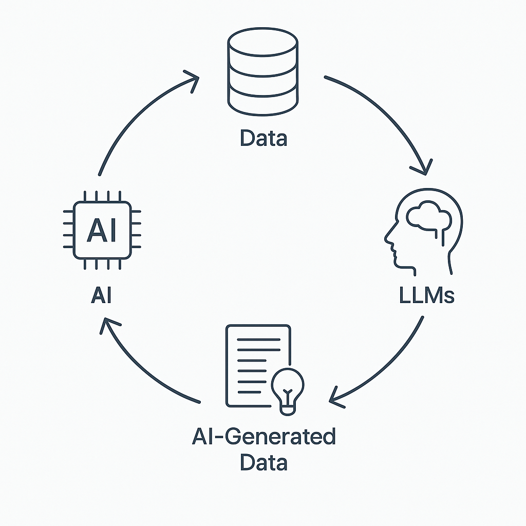
With the rise of Artificial Intelligence (AI) and especially Large Language Models (LLMs) like ChatGPT, Bard, and Claude, the volume of data being generated, consumed, and required for training is skyrocketing.
-
LLMs Need Massive Training Data
-
LLMs generated content is exponential — blogs, reports, summaries, images, audio, and even code.
-
Storage systems must scale horizontally to handle petabytes or more.
-
Traditional databases can’t manage this scale efficiently.
-
Volume impacts data ingestion, processing speed, query performance, and cost.
-
It influences how data is partitioned, replicated, and compressed in distributed systems.
[Avg. reading time: 4 minutes]
Velocity
Velocity refers to the speed at which data is generated, transmitted, and processed. In the era of Big Data, it’s not just about handling large volumes of data, but also about managing the continuous and rapid flow of data in real-time or near real-time.
High-velocity data comes from various sources such as:
- Social Media Platforms: Tweets, posts, likes, and shares occurring every second.
- Sensor Networks: IoT devices transmitting data continuously.
- Financial Markets: Real-time transaction data and stock price updates.
- Online Streaming Services: Continuous streaming of audio and video content.
- E-commerce Platforms: Real-time tracking of user interactions and transactions.
Managing this velocity requires systems capable of:
- Real-Time Data Processing: Immediate analysis and response to incoming data.
- Scalability: Handling increasing data speeds without performance degradation.
- Low Latency: Minimizing delays in data processing and response times.
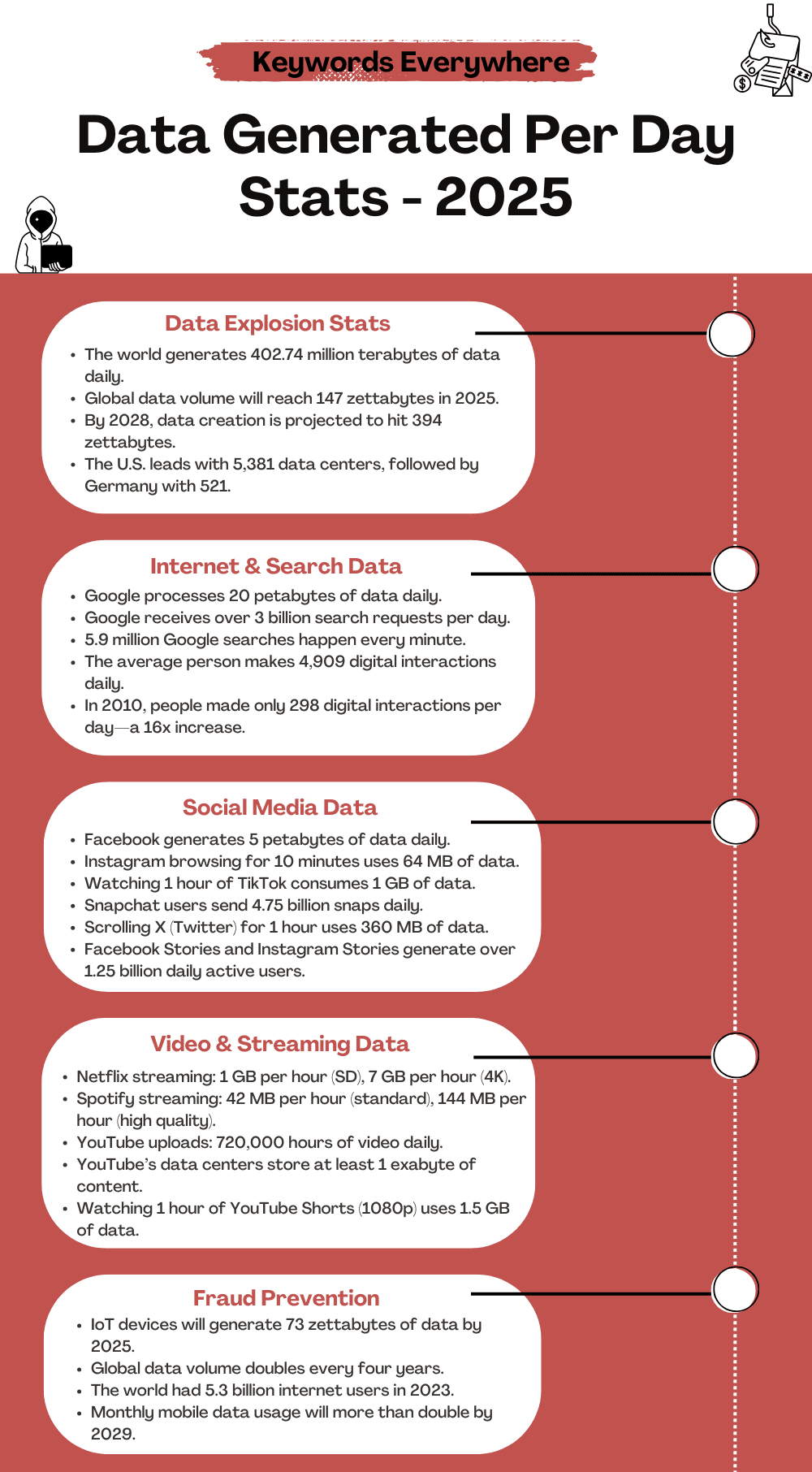 Source1
1: https://keywordseverywhere.com/blog/data-generated-per-day-stats/
[Avg. reading time: 7 minutes]
Veracity
Veracity refers to the trustworthiness, quality, and accuracy of data. In the world of Big Data, not all data is created equal — some may be incomplete, inconsistent, outdated, or even deliberately false. The challenge is not just collecting data, but ensuring it’s reliable enough to make sound decisions.
Why Veracity Matters
-
Poor data quality can lead to wrong insights, flawed models, and bad business decisions.
-
With increasing sources (social media, sensors, web scraping), there’s more noise than ever.
-
Real-world data often comes with missing values, duplicates, biases, or outliers.
Key Dimensions of Veracity in Big Data
| Dimension | Description | Example |
|---|---|---|
| Trustworthiness | Confidence in the accuracy and authenticity of data. | Verifying customer feedback vs. bot reviews |
| Origin | The source of the data and its lineage or traceability. | Knowing if weather data comes from reliable source |
| Completeness | Whether the dataset has all required fields and values. | Missing values in patient health records |
| Integrity | Ensuring the data hasn’t been altered, corrupted, or tampered with during storage or transfer. | Using checksums to validate data blocks |
How to Tackle Veracity Issues
- Data Cleaning: Remove duplicates, correct errors, fill missing values.
- Validation & Verification: Check consistency across sources.
- Data Provenance: Track where the data came from and how it was transformed.
- Bias Detection: Identify and reduce systemic bias in training datasets.
- Robust Models: Build models that can tolerate and adapt to noisy inputs.
Websites & Tools to Generate Sample Data
Highly customizable fake data generator; supports exporting as CSV, JSON, SQL. https://mockaroo.com
Easy UI to create datasets with custom fields like names, dates, numbers, etc. https://www.onlinedatagenerator.com
Apart from this, there are few Data generating libraries.
https://faker.readthedocs.io/en/master/
https://github.com/databrickslabs/dbldatagen
Question?
Is generating fake data good or bad?
When we have real data? why generate fake data?
[Avg. reading time: 3 minutes]
Other V’s in Big Data
| Other V’s | Meaning | Key Question / Use Case |
|---|---|---|
| Value | Business/Customer Impact | What value does this data bring to the business or end users? |
| Visualization | Data Representation | Can the data be visualized clearly to aid understanding and decisions? |
| Viability | Production/Sustainability | Is it viable to operationalize and sustain this data in production systems? |
| Virality | Shareability/Impact | Will the message or insight be effective when shared across channels (e.g., social media)? |
| Version | Data Versioning | Do we need to maintain different versions? Is the cost of versioning justified? |
| Validity | Time-Sensitivity | How long is the data relevant? Will its meaning or utility change over time? |
Example
-
Validity: Zoom usage data from 2020 was valid during lockdown, can that be used for benchmarking?
-
Virality: A meme might go viral on Instagram and not received well in Twitter or LinkedIn.
-
Version: For some master records, we might need versioned data. For simple web traffic counts, maybe not.
#bigdata #otherv #value #version #validity
[Avg. reading time: 7 minutes]
Trending Technologies
Powered by Big Data
Big Data isn’t just about storing and processing huge volumes of information — it’s the engine that drives modern innovation. From healthcare to self-driving cars, Big Data plays a critical role in shaping the technologies we use and depend on every day.
Where Big Data Is Making an Impact
-
Robotics
Enhances learning and adaptive behavior in robots by feeding real-time and historical data into control algorithms. -
Artificial Intelligence (AI)
The heart of AI — machine learning models rely on Big Data to train, fine-tune, and make accurate predictions. -
Internet of Things (IoT)
Millions of devices — from smart thermostats to industrial sensors — generate data every second. Big Data platforms analyze this for real-time insights. -
Internet & Mobile Apps
Collect user behavior data to power personalization, recommendations, and user experience optimization. -
Autonomous Cars & VANETs (Vehicular Networks)
Use sensor and network data for route planning, obstacle avoidance, and decision-making. -
Wireless Networks & 5G
Big Data helps optimize network traffic, reduce latency, and predict service outages before they occur. -
Voice Assistants (Siri, Alexa, Google Assistant)
Depend on Big Data and NLP models to understand speech, learn preferences, and respond intelligently. -
Cybersecurity
Uses pattern detection on massive datasets to identify anomalies, prevent attacks, and detect fraud in real time. -
Bioinformatics & Genomics
Big Data helps decode genetic sequences, enabling personalized medicine and new drug discoveries. Big Data was a game-changer in the development and distribution of COVID-19 vaccineshttps://pmc.ncbi.nlm.nih.gov/articles/PMC9236915/
-
Renewable Energy
Analyzes weather, consumption, and device data to maximize efficiency in solar, wind, and other green technologies. -
Neural Networks & Deep Learning
These advanced AI models require large-scale labeled data for training complex tasks like image recognition or language translation.
Broad Use Areas for Big Data
| Area | Description |
|---|---|
| Data Mining & Analytics | Finding patterns and insights from raw data |
| Data Visualization | Presenting data in a human-friendly, understandable format |
| Machine Learning | Training models that learn from historical data |
#bigdata #technologies #iot #ai #robotics
[Avg. reading time: 6 minutes]
Big Data Concerns
Big Data brings massive potential, but it also introduces ethical, technical, and societal challenges. Below is a categorized view of key concerns and how they can be mitigated.
Privacy, Security & Governance
Concerns
- Privacy: Risk of misuse of sensitive personal data.
- Security: Exposure to cyberattacks and data breaches.
- Governance: Lack of clarity on data ownership and access rights.
Mitigation
- Use strong encryption, anonymization, and secure access controls.
- Conduct regular security audits and staff awareness training.
- Define and enforce data governance policies on ownership, access, and lifecycle.
- Establish consent mechanisms and transparent data usage policies.
Data Quality, Accuracy & Interpretation
Concerns
- Inaccurate, incomplete, or outdated data may lead to incorrect decisions.
- Misinterpretation due to lack of context or domain understanding.
Mitigation
- Implement data cleaning, validation, and monitoring procedures.
- Train analysts to understand data context.
- Use cross-functional teams for balanced analysis.
- Maintain data lineage and proper documentation.
Ethics, Fairness & Bias
Concerns
- Potential for discrimination or unethical use of data.
- Over-reliance on algorithms may overlook human factors.
Mitigation
- Develop and follow ethical guidelines for data usage.
- Perform bias audits and impact assessments regularly.
- Combine data-driven insights with human judgment.
Regulatory Compliance
Concerns
- Complexity of complying with regulations like GDPR, HIPAA, etc.
Mitigation
- Stay current with relevant data protection laws.
- Assign a Data Protection Officer (DPO) to ensure ongoing compliance and oversight.
Environmental and Social Impact
Concerns
- High energy usage of data centers contributes to carbon emissions.
- Digital divide may widen gaps between those who can access Big Data and those who cannot.
Mitigation
- Use energy-efficient infrastructure and renewable energy sources.
- Support data literacy, open data access, and inclusive education initiatives.
#bigdata #concerns #mitigation
[Avg. reading time: 9 minutes]
Big Data Challenges
As organizations adopt Big Data, they face several challenges — technical, organizational, financial, legal, and ethical. Below is a categorized overview of these challenges along with effective mitigation strategies.
1. Data Storage & Management
Challenge:
Efficiently storing and managing ever-growing volumes of structured, semi-structured, and unstructured data.
Mitigation:
- Use scalable cloud storage and distributed file systems like HDFS or Delta Lake.
- Establish data lifecycle policies, retention rules, and metadata catalogs for better management.
2. Data Processing & Real-Time Analytics
Challenges:
- Processing huge datasets with speed and accuracy.
- Delivering real-time insights for time-sensitive decisions.
Mitigation:
- Leverage tools like Apache Spark, Flink, and Hadoop for distributed processing.
- Use streaming platforms like Kafka or Spark Streaming.
- Apply parallel and in-memory processing where possible.
3. Data Integration & Interoperability
Challenge:
Bringing together data from diverse sources, formats, and systems into a unified view.
Mitigation:
- Implement ETL/ELT pipelines, data lakes, and integration frameworks.
- Apply data transformation and standardization best practices.
4. Privacy, Security & Compliance
Challenges:
- Preventing data breaches and unauthorized access.
- Adhering to global and regional data regulations (e.g., GDPR, HIPAA, CCPA).
Mitigation:
- Use encryption, role-based access controls, and audit logging.
- Conduct regular security assessments and appoint a Data Protection Officer (DPO).
- Stay current with evolving regulations and enforce compliance frameworks.
5. Data Quality & Trustworthiness
Challenge:
Ensuring that data is accurate, consistent, timely, and complete.
Mitigation:
- Use data validation, cleansing tools, and automated quality checks.
- Monitor for data drift and inconsistencies in real time.
- Maintain data provenance for traceability.
6. Skill Gaps & Talent Shortage
Challenge:
A lack of professionals skilled in Big Data technologies, analytics, and data engineering.
Mitigation:
- Invest in upskilling programs, certifications, and academic partnerships.
- Foster a culture of continuous learning and data literacy across roles.
7. Cost & Resource Management
Challenge:
Managing the high costs associated with storing, processing, and analyzing large-scale data.
Mitigation:
- Optimize workloads using cloud-native autoscaling and resource tagging.
- Use open-source tools where possible.
- Monitor and forecast data usage to control spending.
8. Scalability & Performance
Challenge:
Keeping up with growing data volumes and system demands without compromising performance.
Mitigation:
- Design for horizontal scalability using microservices and cloud-native infrastructure.
- Implement load balancing, data partitioning, and caching strategies.
9. Ethics, Governance & Transparency
Challenges:
- Managing bias, fairness, and responsible data usage.
- Ensuring transparency in algorithms and decisions.
Mitigation:
- Establish data ethics policies and review boards.
- Perform regular audits and impact assessments.
- Clearly communicate how data is collected, stored, and used.
#bigdata #ethics #storage #realtime #interoperability #privacy #dataquality
[Avg. reading time: 9 minutes]
Data Integration
Data integration in the Big Data ecosystem differs significantly from traditional Relational Database Management Systems (RDBMS). While traditional systems rely on structured, predefined workflows, Big Data emphasizes scalability, flexibility, and performance.
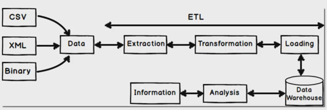
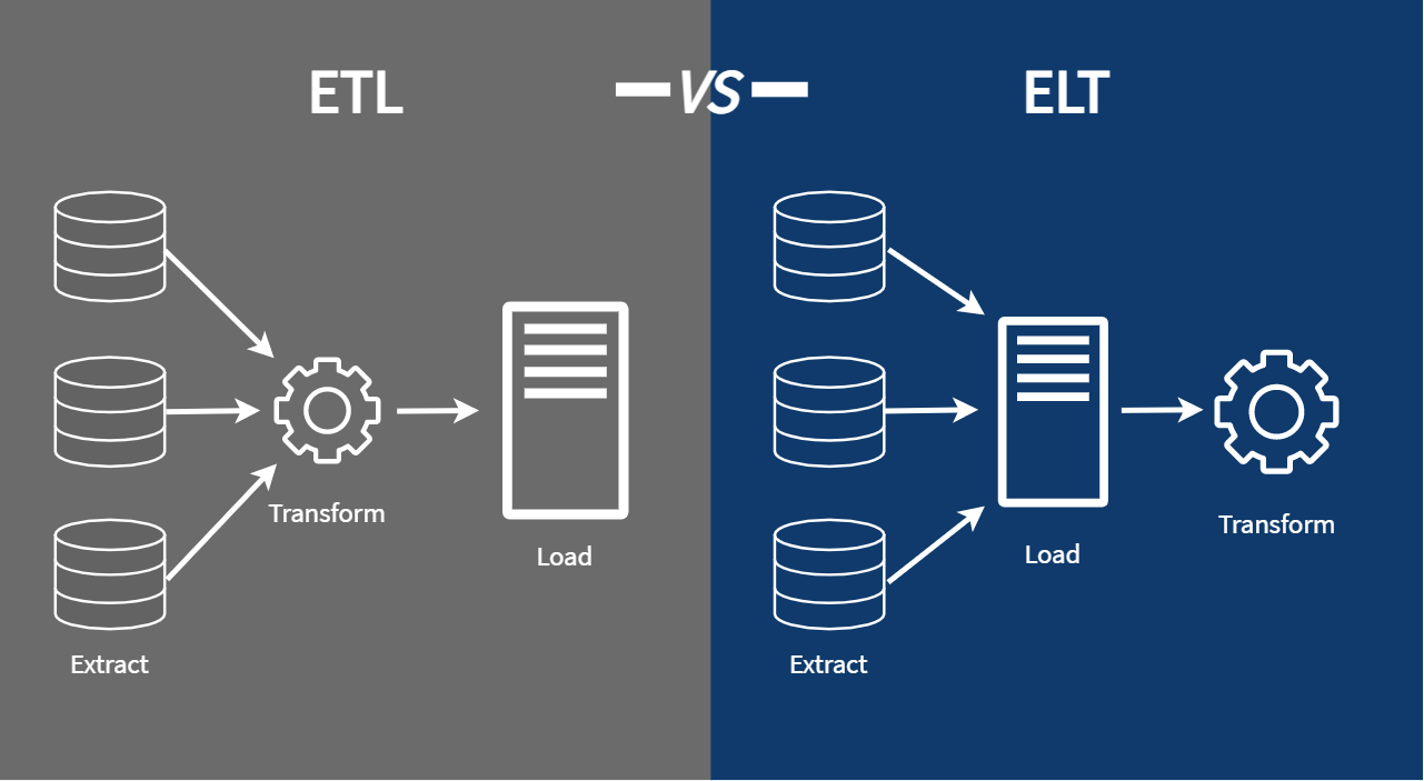
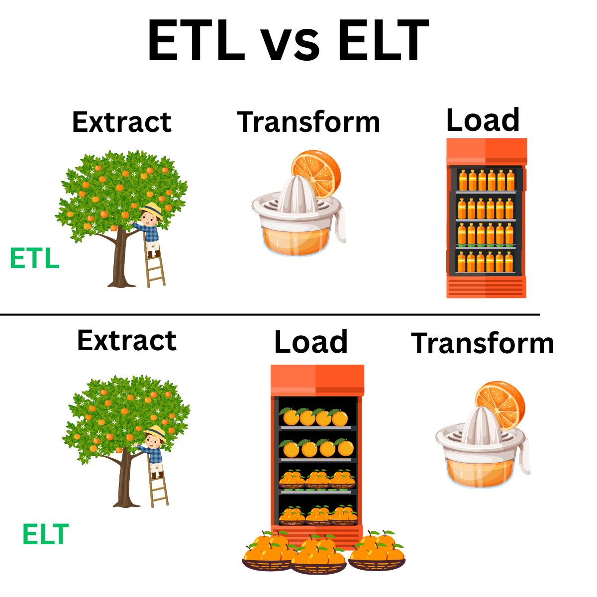
ETL: Extract Transform Load
ETL is a traditional data integration approach used primarily with RDBMS technologies such as MySQL, SQL Server, and Oracle.
Workflow
- Extract data from source systems.
- Transform it into the required format.
- Load it into the target system (e.g., a data warehouse).
ETL Tools
- SSIS / SSDT – SQL Server Integration Services / Data Tools
- Pentaho Kettle – Open-source ETL platform
- Talend – Data integration and transformation platform
- Benetl – Lightweight ETL for MySQL and PostgreSQL
ETL tools are well-suited for batch processing and structured environments but may struggle with scale and unstructured data.
src 1
src 2
ELT: Extract Load Transform
ELT is the modern, Big Data-friendly approach. Instead of transforming data before loading, ELT prioritizes loading raw data first and transforming later.
Benefits
- Immediate ingestion of all types of data (structured or unstructured)
- Flexible transformation logic, applied post-load
- Faster load times and higher throughput
- Reduced operational overhead for loading processes
Challenges
- Security blind spots may arise from loading raw data upfront
- Compliance risks due to delayed transformation (HIPAA, GDPR, etc.)
- High storage costs if raw data is stored unfiltered in cloud/on-prem systems
ELT is ideal for data lakes, streaming, and cloud-native architectures.
Typical Big Data Flow
Raw Data → Cleansed Data → Data Processing → Data Warehousing → ML / BI / Analytics
- Raw Data: Initial unprocessed input (logs, JSON, CSV, APIs, sensors)
- Cleansed Data: Cleaned and standardized
- Processing: Performed through tools like Spark, DLT, or Flink
- Warehousing: Data is stored in structured formats (e.g., Delta, Parquet)
- Usage: Data is consumed by ML models, dashboards, or analysts
Each stage involves pipelines, validations, and metadata tracking.
#etl #elt #pipeline #rawdata #datalake
1: Leanmsbitutorial.com
2: https://towardsdatascience.com/how-i-redesigned-over-100-etl-into-elt-data-pipelines-c58d3a3cb3c
[Avg. reading time: 9 minutes]
Scaling & Distributed Systems
Scalability is a critical factor in Big Data and cloud computing. As workloads grow, systems must adapt.
There are two main ways to scale infrastructure:
vertical scaling and horizontal scaling. These often relate to how distributed systems are designed and deployed.
Vertical Scaling (Scaling Up)
Vertical scaling means increasing the capacity of a single machine.
Like upgrading your personal computer — adding more RAM, a faster CPU, or a bigger hard drive.
Pros:
- Simple to implement
- No code or architecture changes needed
- Good for monolithic or legacy applications
Cons:
- Hardware has physical limits
- Downtime may be required during upgrades
- More expensive hardware = diminishing returns
Used In:
- Traditional RDBMS
- Standalone servers
- Small-scale workloads
Horizontal Scaling (Scaling Out)
Horizontal scaling means adding more machines (nodes) to handle the load collectively.
Like hiring more team members instead of just working overtime yourself.
Pros:
- More scalable: Keep adding nodes as needed
- Fault tolerant: One machine failure doesn’t stop the system
- Supports distributed computing
Cons:
- More complex to configure and manage
- Requires load balancing, data partitioning, and synchronization
- More network overhead
Used In:
- Distributed databases (e.g., Cassandra, MongoDB)
- Big Data platforms (e.g., Hadoop, Spark)
- Cloud-native applications (e.g., Kubernetes)
Distributed Systems
A distributed system is a network of computers that work together to perform tasks. The goal is to increase performance, availability, and fault tolerance by sharing resources across machines.
Analogy:
A relay team where each runner (node) has a specific part of the race, but success depends on teamwork.
Key Features of Distributed Systems
| Feature | Description |
|---|---|
| Concurrency | Multiple components can operate at the same time independently |
| Scalability | Easily expand by adding more nodes |
| Fault Tolerance | If one node fails, others continue to operate with minimal disruption |
| Resource Sharing | Nodes share tasks, data, and workload efficiently |
| Decentralization | No single point of failure; avoids bottlenecks |
| Transparency | System hides its distributed nature from users (location, access, replication) |
Horizontal Scaling vs. Distributed Systems
| Aspect | Horizontal Scaling | Distributed System |
|---|---|---|
| Definition | Adding more machines (nodes) to handle workload | A system where multiple nodes work together as one unit |
| Goal | To increase capacity and performance by scaling out | To coordinate tasks, ensure fault tolerance, and share resources |
| Architecture | Not necessarily distributed | Always distributed |
| Coordination | May not require nodes to communicate | Requires tight coordination between nodes |
| Fault Tolerance | Depends on implementation | Built-in as a core feature |
| Example | Load-balanced web servers | Hadoop, Spark, Cassandra, Kafka |
| Storage/Processing | Each node may handle separate workloads | Nodes often share or split workloads and data |
| Use Case | Quick capacity boost (e.g., web servers) | Large-scale data processing, distributed storage |
Vertical scaling helps improve single-node power, while horizontal scaling enables distributed systems to grow flexibly. Most modern Big Data systems rely on horizontal scaling for scalability, reliability, and performance.
#scaling #vertical #horizontal #distributed
[Avg. reading time: 9 minutes]
CAP Theorem
 src 1
src 1
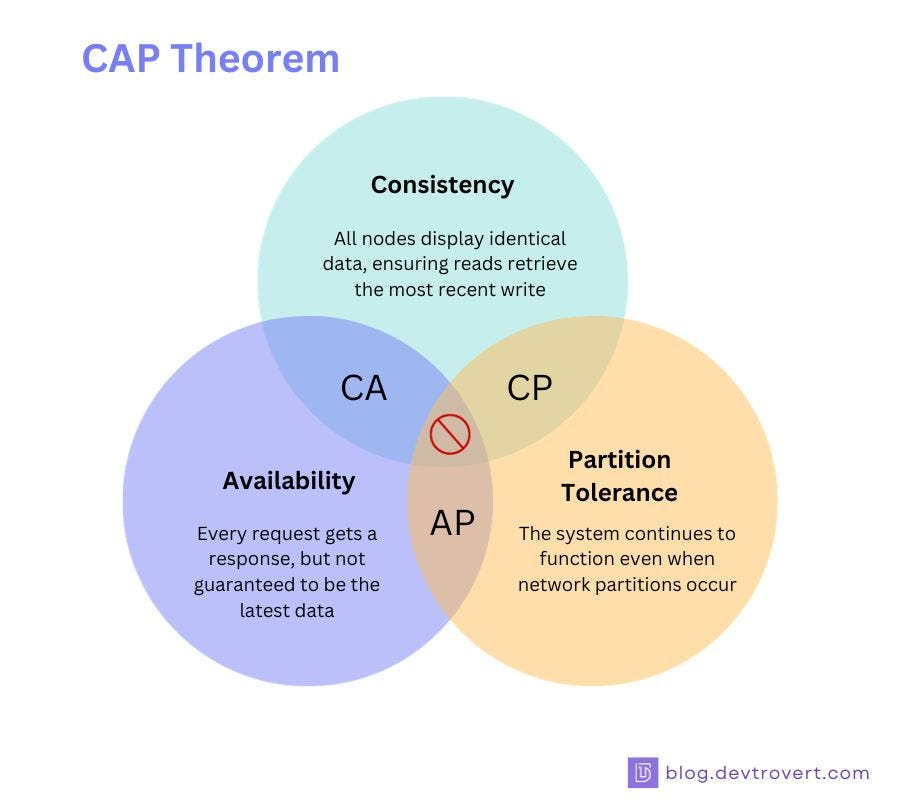
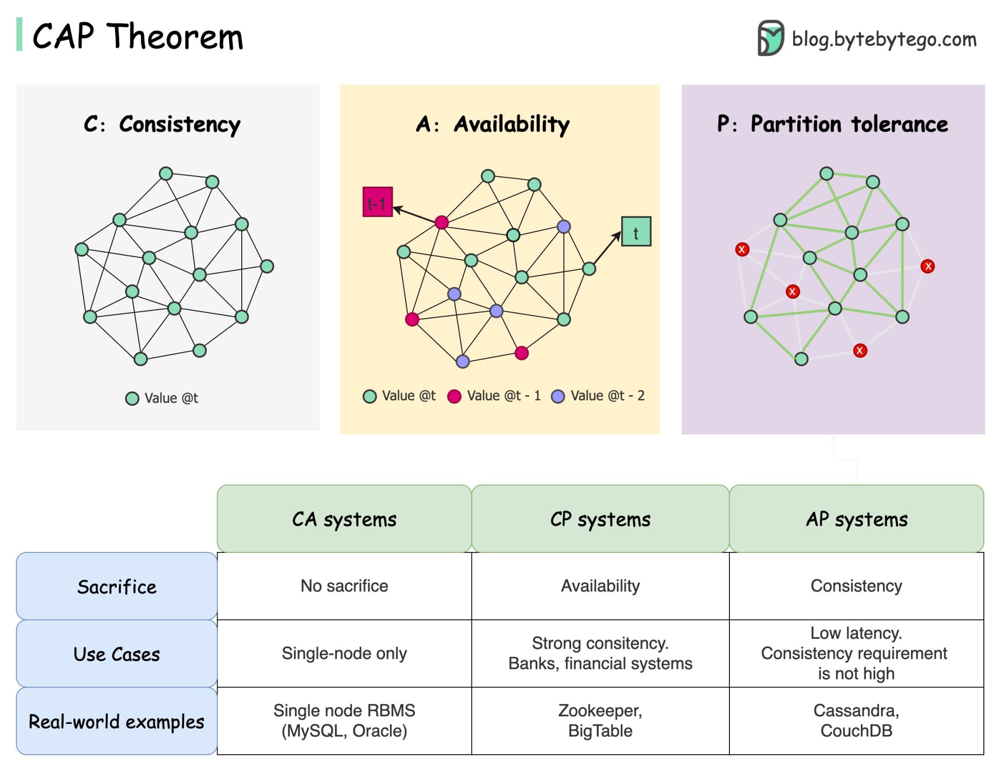
The CAP Theorem is a fundamental concept in distributed computing. It states that in the presence of a network partition, a distributed system can guarantee only two out of the following three properties:
The Three Components
-
Consistency (C)
Every read receives the most recent write or an error.
Example: If a book’s location is updated in a library system, everyone querying the catalog should see the updated location immediately. -
Availability (A)
Every request receives a (non-error) response, but not necessarily the most recent data.
Example: Like a convenience store that’s always open, even if they occasionally run out of your favorite snack. -
Partition Tolerance (P)
The system continues to function despite network failures or communication breakdowns.
Example: A distributed team in different rooms that still works, even if their intercom fails.
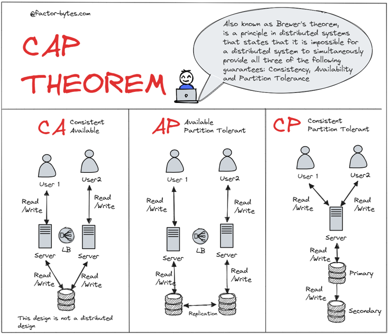
What the CAP Theorem Means
You can only pick two out of three:
| Guarantee Combination | Sacrificed Property | Typical Use Case |
|---|---|---|
| CP (Consistency + Partition) | Availability | Banking Systems, RDBMS |
| AP (Availability + Partition) | Consistency | DNS, Web Caches |
| CA (Consistency + Availability) | Partition Tolerance (Not realistic in distributed systems) | Only feasible in non-distributed systems |
 src 2
src 2
Real-World Examples
CAP Theorem trade-offs can be seen in:
- Social Media Platforms – Favor availability and partition tolerance (AP)
- Financial Systems – Require consistency and partition tolerance (CP)
- IoT Networks – Often prioritize availability and partition tolerance (AP)
- eCommerce Platforms – Mix of AP and CP depending on the service
- Content Delivery Networks (CDNs) – Strongly AP-focused for high availability and responsiveness
 src 3
src 3
graph TD
    A[Consistency]
    B[Availability]
    C[Partition Tolerance]

    A -- CP System --> C
    B -- AP System --> C
    A -- CA System --> B

    subgraph CAP Triangle
        A
        B
        C
    end
This diagram shows that you can choose only two at a time:
- CP (Consistency + Partition Tolerance): e.g., traditional databases
- AP (Availability + Partition Tolerance): e.g., DNS, Cassandra
- CA is only theoretical in a distributed environment (it fails when partition occurs)
In distributed systems, network partitions are unavoidable. The CAP Theorem helps us choose which trade-off makes the most sense for our use case.
#cap #consistency #availability #partitiontolerant
1: blog.devtrovert.com
2: Factor-bytes.com
3: blog.bytebytego.com
[Avg. reading time: 6 minutes]
Optimistic concurrency
Optimistic Concurrency is a concurrency control strategy used in databases and distributed systems that allows multiple users or processes to access the same data simultaneously—without locking resources.
Instead of preventing conflicts upfront by using locks, it assumes that conflicts are rare. If a conflict does occur, it’s detected after the operation, and appropriate resolution steps (like retries) are taken.
How It Works
- Multiple users/processes read and attempt to write to the same data.
- Instead of using locks, each update tracks the version or timestamp of the data.
- When writing, the system checks if the data has changed since it was read.
- If no conflict, the write proceeds.
- If conflict detected, the system throws an exception or prompts a retry.
Let’s look at a simple example:
Sample inventory Table
| item_id | item_nm | stock |
|---------|---------|-------|
|    1    | Apple   |  10   |
|    2    | Orange  |  20   |
|    3    | Banana  |  30   |
Imagine two users, UserA and UserB, trying to update the apple stock simultaneously.
User A’s update:
UPDATE inventory SET stock = stock + 5 WHERE item_id = 1;
User B’s update:
UPDATE inventory SET stock = stock - 3 WHERE item_id = 1;
- Both updates execute concurrently without locking the table.
- After both operations, system checks for version conflicts.
- If there’s no conflict, the changes are merged.
New price of Apple stock = 10 + 5 - 3 = 12
- If there was a conflicting update (e.g., both changed the same field from different base versions), one update would fail, and the user must retry the transaction.
Optimistic Concurrency Is Ideal When
| Condition | Explanation |
|---|---|
| Low write contention | Most updates happen on different parts of data |
| Read-heavy, write-light systems | Updates are infrequent or less overlapping |
| High performance is critical | Avoiding locks reduces wait times |
| Distributed systems | Locking is expensive and hard to coordinate |
[Avg. reading time: 6 minutes]
Eventual consistency
Eventual consistency is a consistency model used in distributed systems (like NoSQL databases and distributed storage) where updates to data may not be immediately visible across all nodes. However, the system guarantees that all replicas will eventually converge to the same state — given no new updates are made.
Unlike stronger models like serializability or linearizability, eventual consistency prioritizes performance and availability, especially in the face of network latency or partitioning.
Simple Example: Distributed Key-Value Store
Imagine a distributed database with three nodes: Node A, Node B, and Node C. All store the value for a key called "item_stock":
Node A: item_stock = 10
Node B: item_stock = 10
Node C: item_stock = 10
Now, a user sends an update to change item_stock to 15, and it reaches only Node A initially:
Node A: item_stock = 15
Node B: item_stock = 10
Node C: item_stock = 10
At this point, the system is temporarily inconsistent. Over time, the update propagates:
Node A: item_stock = 15
Node B: item_stock = 15
Node C: item_stock = 10
Eventually, all nodes reach the same value:
Node A: item_stock = 15
Node B: item_stock = 15
Node C: item_stock = 15
Key Characteristics
- Temporary inconsistencies are allowed
- Data will converge across replicas over time
- Reads may return stale data during convergence
- Prioritizes availability and partition tolerance over strict consistency
When to Use Eventual Consistency
Eventual consistency is ideal when:
| Situation | Why It Helps |
|---|---|
| High-throughput, low-latency systems | Avoids the overhead of strict consistency |
| Geo-distributed deployments | Tolerates network delays and partitions |
| Systems with frequent writes | Enables faster response without locking or blocking |
| Availability is more critical than accuracy | Keeps services running even during network issues |
[Avg. reading time: 6 minutes]
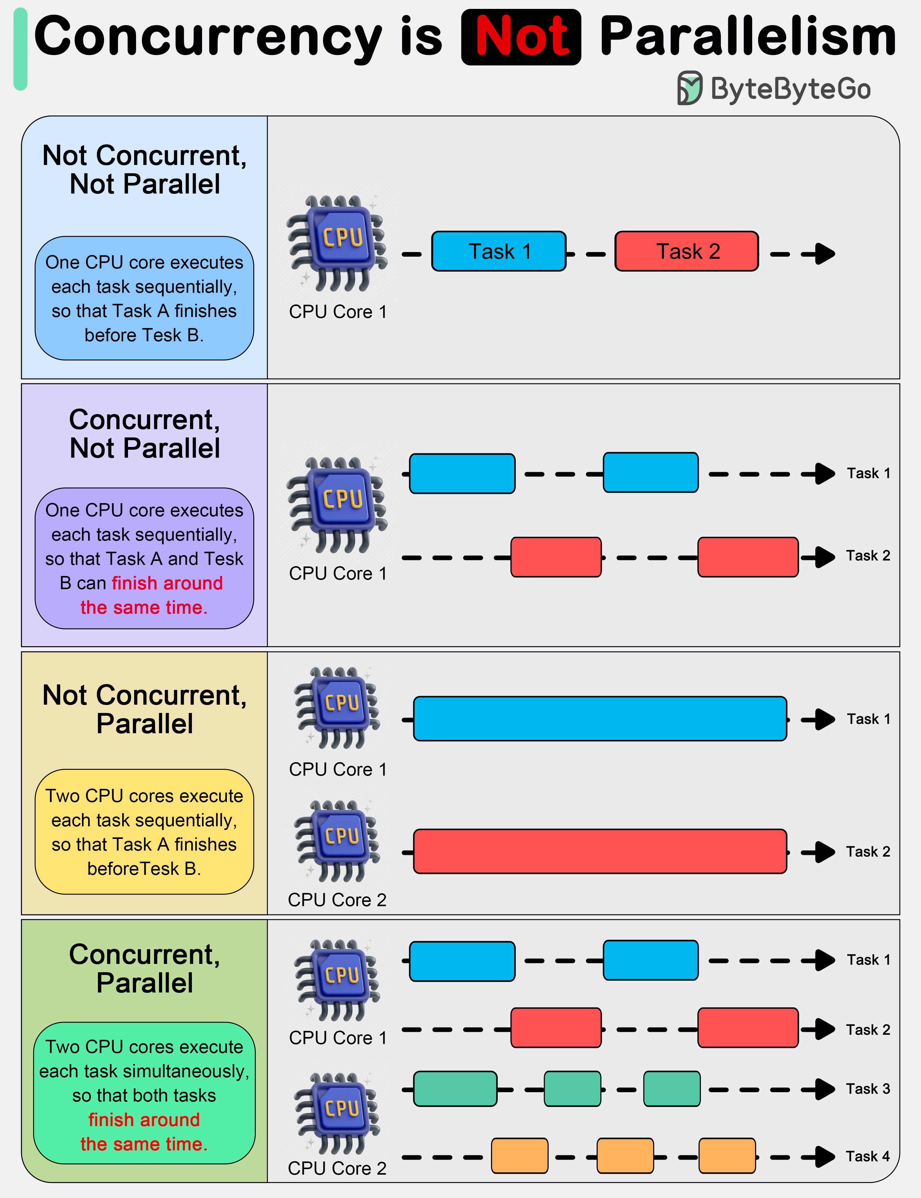
Concurrent vs. Parallel
Understanding the difference between concurrent and parallel programming is key when designing efficient, scalable applications — especially in distributed and multi-core systems.
Concurrent Programming
Concurrent programming is about managing multiple tasks at once, allowing them to make progress without necessarily executing at the same time.
- Tasks overlap in time.
- Focuses on task coordination, not simultaneous execution.
- Often used in systems that need to handle many events or users, like web servers or GUIs.
Key Traits
- Enables responsive programs (non-blocking)
- Utilizes a single core or limited resources efficiently
- Requires mechanisms like threads, coroutines, or async/await
Parallel Programming
Parallel programming is about executing multiple tasks simultaneously, typically to speed up computation.
- Tasks run at the same time, often on multiple cores.
- Focuses on performance and efficiency.
- Common in high-performance computing, such as scientific simulations or data processing.
Key Traits
- Requires multi-core CPUs or GPUs
- Ideal for data-heavy workloads
- Uses multithreading, multiprocessing, or vectorization
Analogy: Cooking in a Kitchen
Concurrent Programming

One chef is working on multiple dishes. While a pot is simmering, the chef chops vegetables for the next dish. Tasks overlap, but only one is actively running at a time.
Parallel Programming

A team of chefs in a large kitchen, each cooking a different dish at the same time. Multiple dishes are actively being cooked simultaneously, speeding up the overall process.
Summary Table
| Feature | Concurrent Programming | Parallel Programming |
|---|---|---|
| Task Timing | Tasks overlap, but not necessarily at once | Tasks run simultaneously |
| Focus | Managing multiple tasks efficiently | Improving performance through parallelism |
| Execution Context | Often single-core or logical thread | Multi-core, multi-threaded or GPU-based |
| Tools/Mechanisms | Threads, coroutines, async I/O | Threads, multiprocessing, SIMD, OpenMP |
| Example Use Case | Web servers, I/O-bound systems | Scientific computing, big data, simulations |
#concurrent #parallelprogramming
[Avg. reading time: 3 minutes]
General-Purpose Language (GPL)
What is a GPL?
A GPL is a programming language designed to write software in multiple problem domains. It is not limited to a particular application area.
Swiss Army Knife

Examples
- Python – widely used in ML, web, scripting, automation.
- Java – enterprise applications, Android, backend.
- C++ – system programming, game engines.
- Rust – performance + memory safety.
- JavaScript – web front-end & server-side with Node.js.
Use Cases
- Building web apps (backend/frontend).
- Developing AI/ML pipelines.
- Writing system software and operating systems.
- Implementing data processing frameworks (e.g., Apache Spark in Scala).
- Creating mobile and desktop applications.
Why Use GPL?
- Flexibility to work across domains.
- Rich standard libraries and ecosystems.
- Ability to combine different kinds of tasks (e.g., networking + ML).
[Avg. reading time: 4 minutes]
DSL
A DSL is a programming or specification language dedicated to a particular problem domain, a particular problem representation technique, and/or a particular solution technique.

Examples
- SQL – querying and manipulating relational databases.
- HTML – for structuring content on the web.
- R – statistical computing and graphics.
- Makefiles – for building projects.
- Regular Expressions – for pattern matching.
- Markdown (READ.md or https://stackedit.io/app#)
- Mermaid - Mermaid (https://mermaid.live/)
Use Cases
- Building data pipelines (e.g., dbt, Airflow DAGs).
- Writing infrastructure-as-code (e.g., Terraform HCL).
- Designing UI layout (e.g., QML for Qt UI design).
- IoT rule engines (e.g., IFTTT or Node-RED flows).
- Statistical models using R.
Why Use DSL?
- Shorter, more expressive code in the domain.
- Higher-level abstractions.
- Reduced risk of bugs for domain experts.
Optional Challenge: Build Your Own DSL!
Design your own mini Domain-Specific Language (DSL)! You can keep it simple.
- Start with a specific problem.
- Create your own syntax that feels natural to all.
- Try few examples and ask your friends to try.
- Try implementing a parser using your favourite GPL.
[Avg. reading time: 4 minutes]
Popular Big Data Tools & Platforms
Big Data ecosystems rely on a wide range of tools and platforms for data processing, real-time analytics, streaming, and cloud-scale storage. Here’s a list of some widely used tools categorized by functionality:
Distributed Processing Engines
- Apache Spark – Unified analytics engine for large-scale data processing; supports batch, streaming, and ML.
- Apache Flink – Framework for stateful computations over data streams with real-time capabilities.
Real-Time Data Streaming
- Apache Kafka – Distributed event streaming platform for building real-time data pipelines and streaming apps.
Log & Monitoring Stack
- ELK Stack (Elasticsearch, Logstash, Kibana) – Searchable logging and visualization suite for real-time analytics.
Cloud-Based Platforms
- AWS (Amazon Web Services) – Scalable cloud platform offering Big Data tools like EMR, Redshift, Kinesis, and S3.
- Azure – Microsoft’s cloud platform with tools like Azure Synapse, Data Lake, and Event Hubs.
- GCP (Google Cloud Platform) – Offers BigQuery, Dataflow, Pub/Sub for large-scale data analytics.
- Databricks – Unified data platform built around Apache Spark with powerful collaboration and ML features.
- Snowflake – Cloud-native data warehouse known for performance, elasticity, and simplicity.
#bigdata #tools #cloud #kafka #spark
[Avg. reading time: 3 minutes]
NoSQL Database Types
NoSQL databases are optimized for flexibility, scalability, and performance, making them ideal for Big Data and real-time applications. They are categorized based on how they store and access data:
Key-Value Stores
Store data as simple key-value pairs. Ideal for caching, session storage, and high-speed lookups.
- Redis
- Amazon DynamoDB
Columnar Stores
Store data in columns rather than rows, optimized for analytical queries and large-scale batch processing.
- Apache HBase
- Apache Cassandra
- Amazon Redshift
Document Stores
Store semi-structured data like JSON or BSON documents. Great for flexible schemas and content management systems.
- MongoDB
- Amazon DocumentDB
Graph Databases
Use nodes and edges to represent and traverse relationships between data. Ideal for social networks, recommendation engines, and fraud detection.
- Neo4j
- Amazon Neptune
Tip: Choose the NoSQL database type based on your data access patterns and application needs.
Not all NoSQL databases solve the same problem.
#nosql #keyvalue #documentdb #graphdb #columnar
[Avg. reading time: 4 minutes]
Learning Big Data
Learning Big Data goes beyond just handling large datasets. It involves building a foundational understanding of data types, file formats, processing tools, and cloud platforms used to store, transform, and analyze data at scale.
Types of Files & Formats
- Data File Types: CSV, JSON
- File Formats: CSV, TSV, TXT, Parquet
Linux & File Management Skills
- Essential Linux Commands:
ls,cat,grep,awk,sort,cut,sed, etc. - Useful Libraries & Tools:
awk,jq,csvkit,grep– for filtering, transforming, and managing structured data
Data Manipulation Foundations
- Regular Expressions: For pattern matching and advanced string operations
- SQL / RDBMS: Understanding relational data and query languages
- NoSQL Databases: Working with document, key-value, columnar, and graph stores
Cloud Technologies
- Introduction to major platforms: AWS, Azure, GCP
- Services for data storage, compute, and analytics (e.g., S3, EMR, BigQuery)
Big Data Tools & Frameworks
- Tools like Apache Spark, Flink, Kafka, Dask
- Workflow orchestration (e.g., Airflow, DBT, Databricks Workflows)
Miscellaneous Tools & Libraries
- Visualization:
matplotlib,seaborn,Plotly - Data Engineering:
pandas,pyarrow,sqlalchemy - Streaming & Real-time:
Kafka,Spark Streaming,Flume
Tip: Big Data learning is a multi-disciplinary journey. Start small — explore files and formats — then gradually move into tools, pipelines, cloud platforms, and real-time systems.
[Avg. reading time: 5 minutes]
Introduction
Before diving into Data or ML frameworks, it's important to have a clean and reproducible development setup. A good environment makes you:
- Faster: less time fighting dependencies.
- Consistent: same results across laptops, servers, and teammates.
- Confident: tools catch errors before they become bugs.
A consistent developer experience saves hours of debugging. You spend more time solving problems, less time fixing environments.
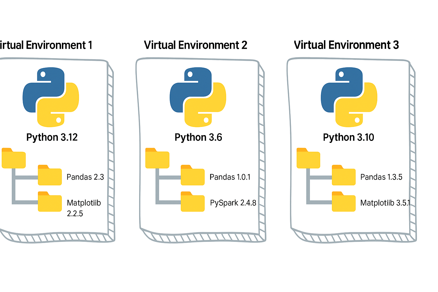
Python Virtual Environment
- A virtual environment is like a sandbox for Python.
- It isolates your project’s dependencies from the global Python installation.
- Easy to manage different versions of library.
- Must depend on requirements.txt, it has to be managed manually.
Without it, installing one package for one project may break another project.
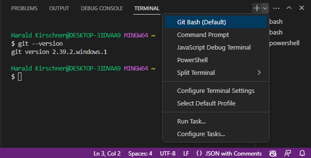
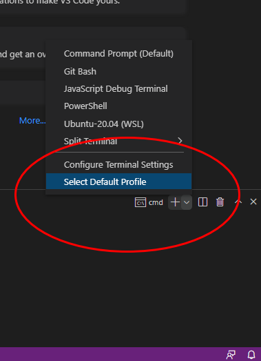
Open the CMD prompt (Windows)
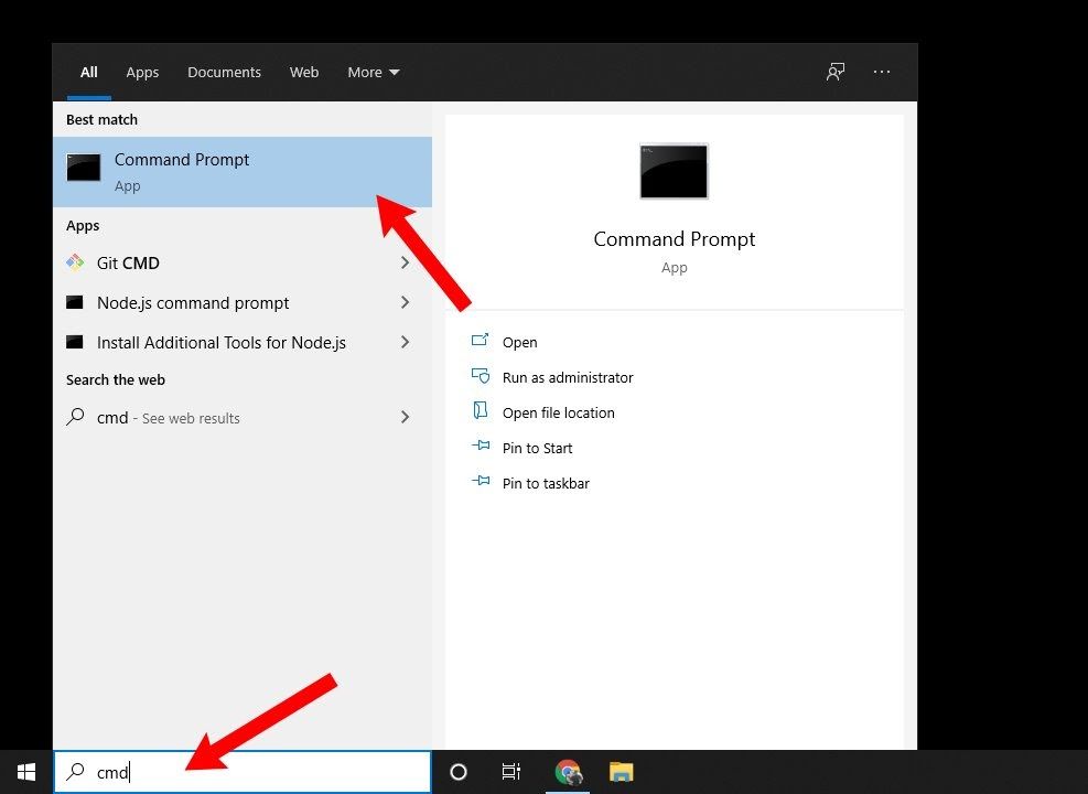
Open the Terminal (Mac)

# Step 0: Create a project folder under your Home folder.

mkdir project

cd project


# Step 1: Create a virtual environment
python -m venv myenv

# Step 2: Activate it
# On Mac/Linux:
source myenv/bin/activate

# On Windows:
myenv\Scripts\activate.bat

# Step 3: Install packages (they go inside `myenv`, not global)
pip install faker

# Step 4: Open Python
python

# Step 5: Verify

import sys

sys.prefix

sys.base_prefix

# Step 6: Run this sample

from faker import Faker
fake = Faker()
fake.name()

# Step 6: Close Python (Control + Z)

# Step 7: Deactivate the venv when done

deactivate
As a next step, you can either use Poetry or UV as your package manager.
#venv #python #uv #poetry developer_tools
[Avg. reading time: 6 minutes]
Poetry
A Dependency & Environment Manager
Poetry simplifies dependency management and packaging in Python projects.
Create a new project:
poetry new helloworld
Sample layout of the directory structure
helloworld/
├── pyproject.toml
├── README.md
├── helloworld/
│   └── __init__.py
└── tests/
    └── __init__.py
- Navigate to your project directory
cd helloworld
Windows Users (Recommended Approach)
Working with Virtual Environments
- Create and activate a virtual environment:
poetry env activate
- Get Virtual Python Interpreter info, to verify the base Python vs Poetry env
poetry env info
Or Use this one line.
poetry env use $(poetry env info -e)
- Verify the Virtual env libraries. You will notice only pip.
poetry run pip list
- Add project dependencies:
poetry add faker
- Create a main.py under src/hellworld/ (subfolder)
main.py
from faker import Faker
fake = Faker()
print(fake.name())
- Run program
poetry run python src/helloworld/main.py
Managing Your Project
- View all installed dependencies:
poetry show
- Update dependencies:
poetry update
- Remove a dependency:
poetry remove package-name
Key Benefits
- Simplified Environment Management
- Poetry automatically creates and manages virtual environments
- No need to manually manage pip and virtualenv
- Clear Dependency Specification
- All dependencies are listed in one file (pyproject.toml)
- Dependencies are automatically resolved to avoid conflicts
- Project Isolation
- Each project has its own dependencies
- Prevents conflicts between different projects
- Easy Distribution
- Package your project with a single command:
poetry build
Publish to PyPI when ready:
poetry publish
Best Practices
- Always activate virtual environment before working on project
- Keep pyproject.toml updated with correct dependencies
- Use version constraints wisely
- Commit both pyproject.toml and poetry.lock files to version control

#python #poetry #ruff #lint #mypy
[Avg. reading time: 3 minutes]
UV
Dependency & Environment Manager
- Written in Rust.
- Syntax is lightweight.
- Automatic Virtual environment creation.
Create a new project:
# Initialize a new uv project
uv init uv_helloworld
Sample layout of the directory structure
.
├── main.py
├── pyproject.toml
├── README.md
└── uv.lock
# Change directory
cd uv_helloworld

# # Create a virtual environment myproject
# uv venv myproject

# or create a UV project with specific version of Python

# uv venv myproject --python 3.11

# # Activate the Virtual environment

# source myproject/bin/activate

# # Verify the Virtual Python version

# which python3

# add library (best practice)
uv add faker

# verify the list of libraries under virtual env
uv tree

# To find the list of libraries inside Virtual env

uv pip list
edit the main.py
from faker import Faker
fake = Faker()
print(fake.name())
uv run main.py
Read More on the differences between UV and Poetry
[Avg. reading time: 12 minutes]
Python Developer Tools
PEP
PEP, or Python Enhancement Proposal, is the official style guide for Python code. It provides conventions and recommendations for writing readable, consistent, and maintainable Python code.
- PEP 8 : Style guide for Python code (most famous).
- PEP 20 : "The Zen of Python" (guiding principles).
- PEP 484 : Type hints (basis for MyPy).
- PEP 517/518 : Build system interfaces (basis for pyproject.toml, used by Poetry/UV).
- PEP 572 : Assignment expressions (the := walrus operator).
- PEP 695 : Type parameter syntax for generics (Python 3.12).
Key Aspects of PEP 8 (Popular ones)
Indentation
- Use 4 spaces per indentation level
- Continuation lines should align with opening delimiter or be indented by 4 spaces.
Line Length
- Limit lines to a maximum of 79 characters.
- For docstrings and comments, limit lines to 72 characters.
Blank Lines
- Use 2 blank lines before top-level functions and class definitions.
- Use 1 blank line between methods inside a class.
Imports
- Imports should be on separate lines.
- Group imports into three sections: standard library, third-party libraries, and local application imports.
- Use absolute imports whenever possible.
# Correct
import os
import sys

# Wrong
import sys, os
Naming Conventions
- Use
snake_casefor function and variable names. - Use
CamelCasefor class names. - Use
UPPER_SNAKE_CASEfor constants. - Avoid single-character variable names except for counters or indices.
Whitespace
- Don’t pad inside parentheses/brackets/braces.
- Use one space around operators and after commas, but not before commas.
- No extra spaces when aligning assignments.
Comments
- Write comments that are clear, concise, and helpful.
- Use complete sentences and capitalize the first word.
- Use # for inline comments, but avoid them where the code is self-explanatory.
Docstrings
- Use triple quotes (""") for multiline docstrings.
- Describe the purpose, arguments, and return values of functions and methods.
Code Layout
- Keep function definitions and calls readable.
- Avoid writing too many nested blocks.
Consistency
- Consistency within a project outweighs strict adherence.
- If you must diverge, be internally consistent.
Linting
Linting is the process of automatically checking your Python code for:
-
Syntax errors
-
Stylistic issues (PEP 8 violations)
-
Potential bugs or bad practices
-
Keeps your code consistent and readable.
-
Helps catch errors early before runtime.
-
Encourages team-wide coding standards.
# Incorrect
import sys, os

# Correct
import os
import sys
# Bad spacing
x= 5+3

# Good spacing
x = 5 + 3
Ruff : Linter and Code Formatter
Ruff is a fast, modern tool written in Rust that helps keep your Python code:
- Consistent (follows PEP 8)
- Clean (removes unused imports, fixes spacing, etc.)
- Correct (catches potential errors)
Install
poetry add ruff
uv add ruff
Verify
ruff --version
ruff --help
example.py
import os, sys

def greet(name):
  print(f"Hello, {name}")

def message(name): print(f"Hi, {name}")

def calc_sum(a, b): return a+b

greet('World')
greet('Ruff')
message('Ruff')
poetry run ruff check example.py
poetry run ruff check example.py --fix

poetry run ruff format example.py --check
poetry run ruff format example.py
OR
uv run ruff check example.py
uv run ruff check example.py --fix
uv run ruff format example.py --check
uv run ruff check example.py
MyPy : Type Checking Tool
mypy is a static type checker for Python. It checks your code against the type hints you provide, ensuring that the types are consistent throughout the codebase.
It primarily focuses on type correctness—verifying that variables, function arguments, return types, and expressions match the expected types.
Install
    poetry add mypy

    or

    uv add mypy

    or

    pip install mypy
sample.py
x = 1
x = 1.0
x = True
x = "test"
x = b"test"

print(x)

def add(a: int, b: int) -> int:
    return a + b

print(add(100, 123))

print(add("hello", "world"))
uv run mypy sample.py

or

poetry run mypy sample.py

or

mypy sample.py
[Avg. reading time: 11 minutes]
DUCK DB
DuckDB is a single file built with no dependencies.
All the great features can be read here https://duckdb.org/
Automatic Parallelism: DuckDB has improved its automatic parallelism capabilities, meaning it can more effectively utilize multiple CPU cores without requiring manual tuning. This results in faster query execution for large datasets.
Parquet File Improvements: DuckDB has improved its handling of Parquet files, both in terms of reading speed and support for more complex data types and compression codecs. This makes DuckDB an even better choice for working with large datasets stored in Parquet format.
Query Caching: Improves the performance of repeated queries by caching the results of previous executions. This can be a game-changer for analytics workloads with similar queries being run multiple times.
How to use DuckDB?
Download the CLI Client
-
Linux).
-
For other programming languages, visit https://duckdb.org/docs/installation/
-
Unzip the file.
-
Open Command / Terminal and run the Executable.
DuckDB in Data Engineering
Download orders.parquet from
https://github.com/duckdb/duckdb-data/releases/download/v1.0/orders.parquet
More files are available here
https://github.com/cwida/duckdb-data/releases/
Open Command Prompt or Terminal
./duckdb
# Create / Open a database

.open ordersdb
Duckdb allows you to read the contents of orders.parquet as is without needing a table. Double quotes around the file name orders.parquet is essential.
describe table "orders.parquet"
Not only this, but it also allows you to query the file as-is. (This feature is similar to one data bricks supports)
select * from "orders.parquet" limit 3;
DuckDB supports CTAS syntax and helps to create tables from the actual file.
show tables;

create table orders  as select * from "orders.parquet";

select count(*) from orders;
DuckDB supports parallel query processing, and queries run fast.
This table has 1.5 million rows, and aggregation happens in less than a second.
select now(); select o_orderpriority,count(*) cnt from orders group by o_orderpriority; select now();
DuckDB also helps to convert parquet files to CSV in a snap. It also supports converting CSV to Parquet.
COPY "orders.parquet" to 'orders.csv' (FORMAT "CSV", HEADER 1);Select * from "orders.csv" limit 3;
It also supports exporting existing Tables to Parquet files.
COPY "orders" to 'neworder.parquet' (FORMAT "PARQUET");
DuckDB supports Programming languages such as Python, R, JAVA, node.js, C/C++.
DuckDB ably supports Higher-level SQL programming such as Macros, Sequences, Window Functions.
Get sample data from Yellow Cab
https://www.nyc.gov/site/tlc/about/tlc-trip-record-data.page
Copy yellow cabs data into yellowcabs folder
create table taxi_trips as select * from "yellowcabs/*.parquet";
SELECT
    PULocationID,
    EXTRACT(HOUR FROM tpep_pickup_datetime) AS hour_of_day,
    AVG(fare_amount) AS avg_fare
FROM
    taxi_trips
GROUP BY
    PULocationID,
    hour_of_day;
Extensions
https://duckdb.org/docs/extensions/overview
INSTALL json;
LOAD json;
select * from demo.json;
describe demo.json;
Load directly from HTTP location
select * from 'https://raw.githubusercontent.com/gchandra10/filestorage/main/sales_100.csv'
#duckdb #singlefiledatabase #parquet #tools #cli
[Avg. reading time: 8 minutes]
JQ
- jq is a lightweight and flexible command-line JSON processor.
- Reads JSON from stdin or a file, applies filters, and writes JSON to stdout.
- Useful when working with APIs, logs, or config files in JSON format.
- Handy tool in Automation.
- Download JQ CLI (Preferred) and learn JQ.
- Use the VSCode Extension and learn JQ.
Download the sample JSON
https://raw.githubusercontent.com/gchandra10/jqtutorial/refs/heads/master/sample_nows.json
Note: As this has no root element, '.' is used.
1. View JSON file in readable format
jq '.' sample_nows.json
2. Read the First JSON element / object
jq 'first(.[])' sample_nows.json
3. Read the Last JSON element
jq 'last(.[])' sample_nows.json
4. Read top 3 JSON elements
jq 'limit(3;.[])' sample_nows.json
5. Read 2nd & 3rd element. Remember, Python has the same format. LEFT Side inclusive, RIGHT Side exclusive
jq '.[2:4]' sample_nows.json
6. Extract individual values. | Pipeline the output
jq '.[] | [.balance,.age]' sample_nows.json
7. Extract individual values and do some calculations
jq '.[] | [.age, 65 - .age]' sample_nows.json
8. Return CSV from JSON
jq '.[] | [.company, .phone, .address] | @csv ' sample_nows.json
9. Return Tab Separated Values (TSV) from JSON
jq '.[] | [.company, .phone, .address] | @tsv ' sample_nows.json
10. Return with custom pipeline delimiter ( | )
jq '.[] | [.company, .phone, .address] | join("|")' sample_nows.json
Pro TIP : Export this result > output.txt and Import to db using bulk import tools like bcp, load data infile
11. Convert the number to string and return | delimited result
jq '.[] | [.balance,(.age | tostring)] | join("|") ' sample_nows.json
12. Process Array return Name (returns as list / array)
jq '.[] | [.friends[].name]' sample_nows.json
or (returns line by line)
jq '[].friends[].name' sample_nows.json
13. Parse multi level values
returns as list / array
jq '.[] | [.name.first, .name.last]' sample_nows.json
returns line by line
jq '.[].name.first, .[].name.last' sample_nows.json
14. Query values based on condition, say .index > 2
jq 'map(select(.index > 2))' sample_nows.json
jq 'map(select(.index > 2)) | .[] | [.index,.balance,.age]' sample_nows.json
15. Sorting Elements
# Sort by Age ASC
jq 'sort_by(.age)' sample_nows.json
# Sort by Age DESC
jq 'sort_by(-.age)' sample_nows.json
# Sort on multiple keys
jq 'sort_by(.age, .index)' sample_nows.json
Use Cases
curl -s https://www.githubstatus.com/api/v2/status.json
curl -s https://www.githubstatus.com/api/v2/status.json | jq '.'
curl -s https://www.githubstatus.com/api/v2/status.json | jq '.status'
#jq #tools #json #parser #cli #automation
[Avg. reading time: 3 minutes]
Introduction to Data Formats
What are Data Formats?
- Data formats define how data is structured, stored, and exchanged between systems.
- In Big Data, the choice of data format is crucial because it affects:
- Storage efficiency
- Processing speed
- Interoperability
- Compression
Why are Data Formats Important in Big Data?
- Big Data often involves massive volumes of data from diverse sources.
- Choosing the right format ensures:
- Efficient data storage
- Faster querying and processing
- Easier integration with analytics frameworks like Spark, Flink, etc.
Data Formats vs. Traditional Database Storage
| Feature | Traditional RDBMS | Big Data Formats |
|---|---|---|
| Storage | Tables with rows and columns | Files/Streams with structured data |
| Schema | Fixed and enforced | Flexible, sometimes schema-on-read |
| Processing | Transactional, ACID | Batch or stream, high throughput |
| Data Model | Relational | Structured, semi-structured, binary |
| Use Cases | OLTP, Reporting | ETL, Analytics, Machine Learning |
[Avg. reading time: 3 minutes]
Common Data Formats
CSV (Comma-Separated Values)
A simple text-based format where each row is a record and columns are separated by commas.
Example:
name,age,city
Rachel,30,New York
Phoebe,25,San Francisco
Use Cases:
- Data exchange between systems
- Lightweight storage
Pros:
- Human-readable
- Easy to generate and parse
Cons:
- No support for nested or complex structures
- No schema enforcement
- Inefficient for very large data
TSV (Tab-Separated Values)
Like CSV but uses tabs instead of commas.
Example:
name    age    city
Rachel   30     New York
Phoebe     25     San Francisco
Use Cases:
Similar to CSV but avoids issues with commas in data
Pros:
- Easy to read and parse
- Handles data with commas
Cons:
- Same as CSV: no schema, no nested data
#bigdata #dataformat #csv #parquet #arrow
[Avg. reading time: 8 minutes]
JSON
Java Script Object Notation.
- This is neither a row-based nor Columnar Format.
- The flexible way to store & share data across systems.
- It's a text file with curly braces & key-value pairs { }
Simplest JSON format
{"id": "1","name":"Rachel"}
Properties
- Language Independent.
- Self-describing and easy to understand.
Basic Rules
- Curly braces to hold the objects.
- Data is represented in Key Value or Name Value pairs.
- Data is separated by a comma.
- The use of double quotes is necessary.
- Square brackets [ ] hold an array of data.
JSON Values
String  {"name":"Rachel"}

Number  {"id":101}

Boolean {"result":true, "status":false}  (lowercase)

Object  {
            "character":{"fname":"Rachel","lname":"Green"}
        }

Array   {
            "characters":["Rachel","Ross","Joey","Chanlder"]
        }

NULL    {"id":null}
Sample JSON Document
{
    "characters": [
        {
            "id" : 1,
            "fName":"Rachel",
            "lName":"Green",
            "status":true
        },
        {
            "id" : 2,
            "fName":"Ross",
            "lName":"Geller",
            "status":true
        },
        {
            "id" : 3,
            "fName":"Chandler",
            "lName":"Bing",
            "status":true
        },
        {
            "id" : 4,
            "fName":"Phebe",
            "lName":"Buffay",
            "status":false
        }
    ]
}
JSON Best Practices
No Hyphen in your Keys.
{"first-name":"Rachel","last-name":"Green"} is not right. ✘
Under Scores Okay
{"first_name":"Rachel","last_name":"Green"} is okay ✓
Lowercase Okay
{"firstname":"Rachel","lastname":"Green"} is okay ✓
Camelcase best
{"firstName":"Rachel","lastName":"Green"} is the best. ✓
Use Cases
-
APIs and Web Services: JSON is widely used in RESTful APIs for sending and receiving data.
-
Configuration Files: Many modern applications and development tools use JSON for configuration.
-
Data Storage: Some NoSQL databases like MongoDB use JSON or BSON (binary JSON) for storing data.
-
Serialization and Deserialization: Converting data to/from a format that can be stored or transmitted.
Python Example
Serialize : Convert Python Object to JSON (Shareable) Format.
DeSerialize : Convert JSON (Shareable) String to Python Object.
import json

def json_serialize(file_name):
    # Python dictionary with Friend's characters
    friends_characters = {
        "characters": [{
            "name": "Rachel Green",
            "job": "Fashion Executive"
        }, {
            "name": "Ross Geller",
            "job": "Paleontologist"
        }, {
            "name": "Monica Geller",
            "job": "Chef"
        }, {
            "name": "Chandler Bing",
            "job": "Statistical Analysis and Data Reconfiguration"
        }, {
            "name": "Joey Tribbiani",
            "job": "Actor"
        }, {
            "name": "Phoebe Buffay",
            "job": "Massage Therapist"
        }]
    }

    print(type(friends_characters), friends_characters)

    print("-" * 200)

    # Serializing json
    json_data = json.dumps(friends_characters, indent=4)
    print(type(json_data), json_data)

    # Saving to a file
    with open(file_name, 'w') as file:
        json.dump(friends_characters, file, indent=4)


def json_deserialize(file_name):
    #file_path = 'friends_characters.json'

    # Open the file and read the JSON content
    with open(file_name, 'r') as file:
        data = json.load(file)
    print(data, type(data))


def main():
    file_name = 'friends_characters.json'
    json_serialize(file_name)
    json_deserialize(file_name)


if __name__ == "__main__":
    print("Starting JSON Serialization...")
    main()
    print("Done!")
#bigdata #dataformat #json #hierarchical
[Avg. reading time: 20 minutes]
Parquet
Parquet is a columnar storage file format optimized for use with Apache Hadoop and related big data processing frameworks. Originally developed by Twitter and Cloudera, Parquet provides a compact and efficient way of storing large, flat datasets.
Best suited for WORM (Write Once, Read Many) workloads.
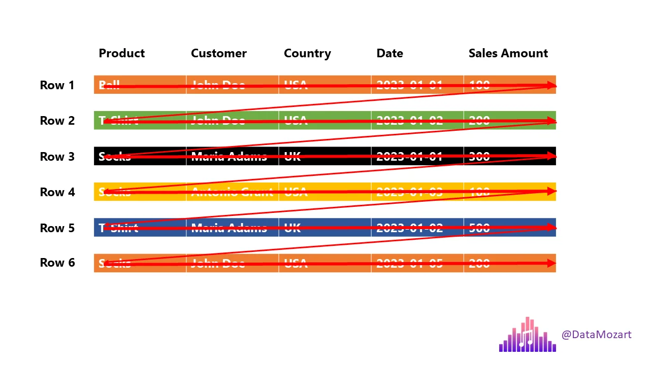
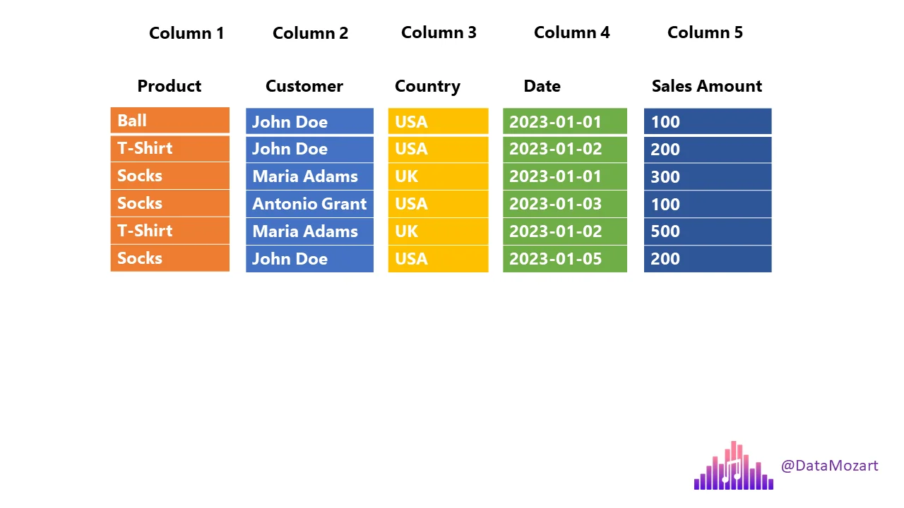
Row Storage
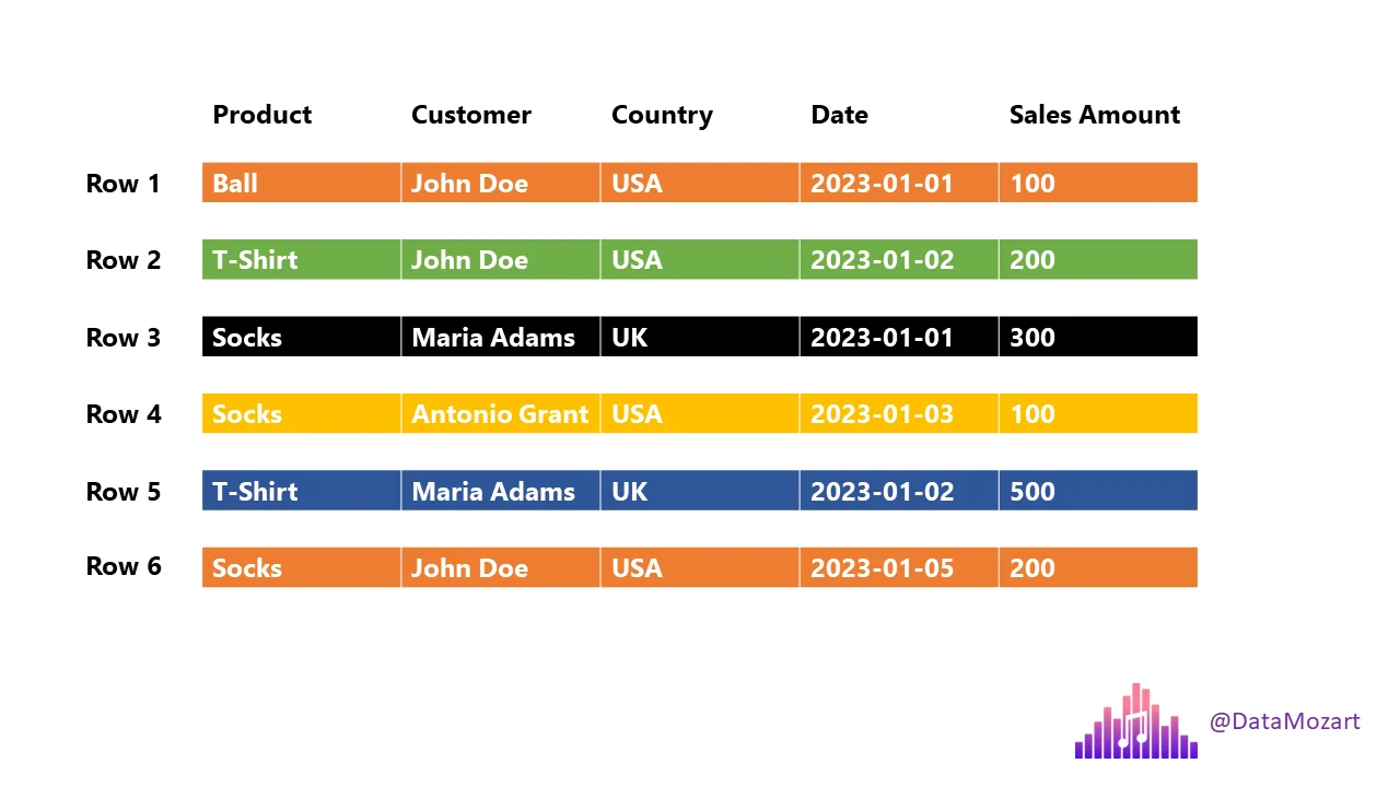
Give me list of Total T-Shirts sold or Customers from UK
It scans the entire dataset.
Columnar Storage
Terms to Know
Projection: Columns that are needed by the query.
select product, country, salesamount from sales;
Here the projections are: product, country & salesamount
Predicate: A filter condition that selects rows.
select product, country, salesamount from sales where country='UK';
Here predicate is where country = 'UK'
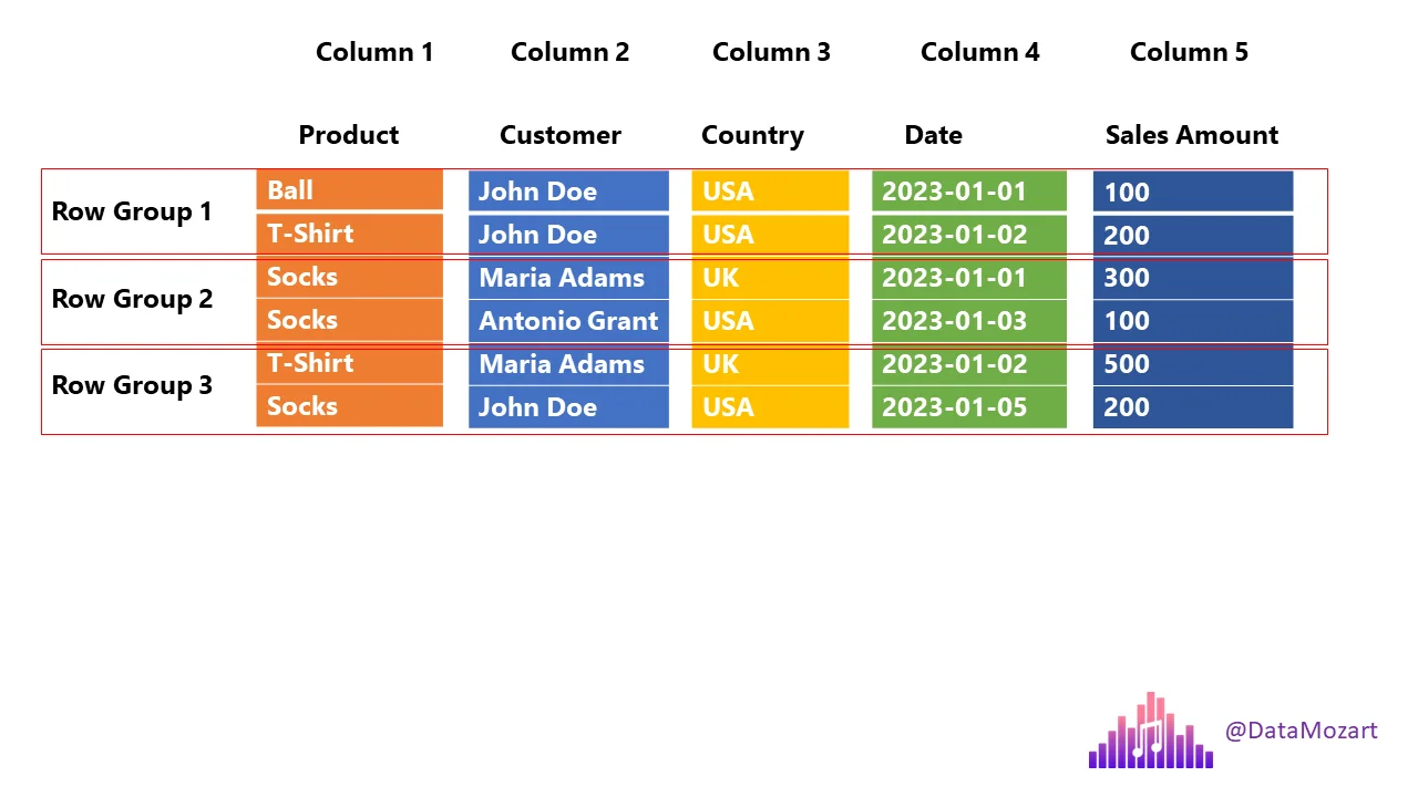
Row Groups in Parquet
-
Parquet divides data into row groups, each containing column chunks for all columns.
-
Horizontal partition—each row group can be processed independently.
-
Row groups enable parallel processing and make it possible to skip unnecessary data using metadata.
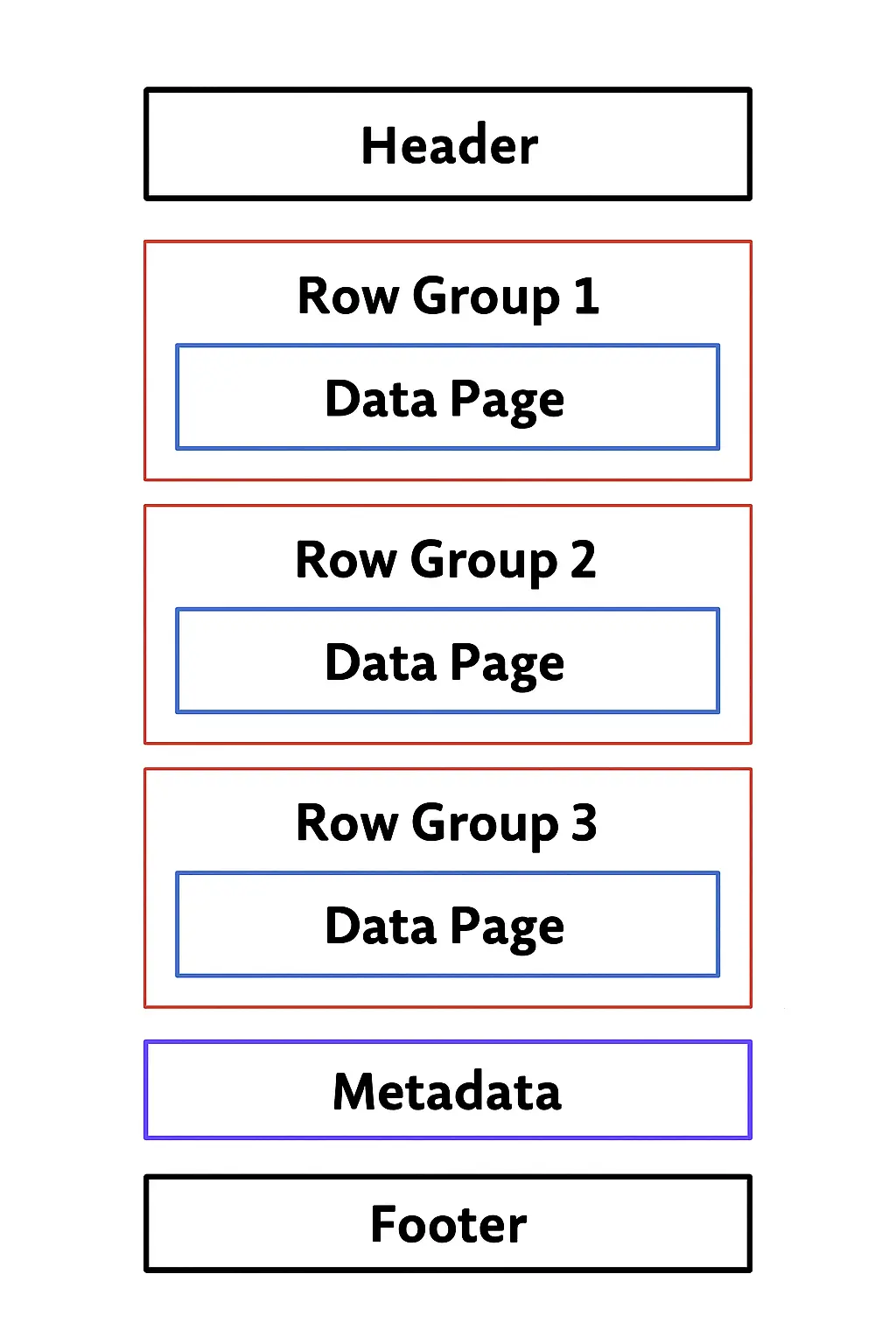
Parquet - Columnar Storage + Row Groups
Parquet File format
Parquet Fileformat Layout {{footnote: https://parquet.apache.org/docs/file-format/}}
Sample Data
| Product | Customer | Country | Date | Sales Amount |
|---|---|---|---|---|
| Ball | John Doe | USA | 2023-01-01 | 100 |
| T-Shirt | John Doe | USA | 2023-01-02 | 200 |
| Socks | Jane Doe | UK | 2023-01-03 | 150 |
| Socks | Jane Doe | UK | 2023-01-04 | 180 |
| T-Shirt | Alex | USA | 2023-01-05 | 120 |
| Socks | Alex | USA | 2023-01-06 | 220 |
Data stored inside Parquet
┌──────────────────────────────────────────────┐
│                File Header                   │
│  ┌────────────────────────────────────────┐  │
│  │ Magic Number: "PAR1"                   │  │
│  └────────────────────────────────────────┘  │
├──────────────────────────────────────────────┤
│                Row Group 1                   │
│  ┌────────────────────────────────────────┐  │
│  │ Column Chunk: Product                  │  │
│  │  ├─ Page 1: Ball, T-Shirt, Socks       │  │
│  └────────────────────────────────────────┘  │
│  ┌────────────────────────────────────────┐  │
│  │ Column Chunk: Customer                 │  │
│  │  ├─ Page 1: John Doe, John Doe, Jane Doe│ │
│  └────────────────────────────────────────┘  │
│  ┌────────────────────────────────────────┐  │
│  │ Column Chunk: Country                  │  │
│  │  ├─ Page 1: USA, USA, UK               │  │
│  └────────────────────────────────────────┘  │
│  ┌────────────────────────────────────────┐  │
│  │ Column Chunk: Date                     │  │
│  │  ├─ Page 1: 2023-01-01, 2023-01-02,    │  │
│  │            2023-01-03                  │  │
│  └────────────────────────────────────────┘  │
│  ┌────────────────────────────────────────┐  │
│  │ Column Chunk: Sales Amount             │  │
│  │  ├─ Page 1: 100, 200, 150              │  │
│  └────────────────────────────────────────┘  │
│  ┌────────────────────────────────────────┐  │
│  │ Row Group Metadata                     │  │
│  │  ├─ Num Rows: 3                        │  │
│  │  ├─ Min/Max per Column:                │  │
│  │     • Product: Ball/T-Shirt/Socks      │  │
│  │     • Customer: Jane Doe/John Doe      │  │
│  │     • Country: UK/USA                  │  │
│  │     • Date: 2023-01-01 to 2023-01-03    │  │
│  │     • Sales Amount: 100 to 200         │  │
│  └────────────────────────────────────────┘  │
├──────────────────────────────────────────────┤
│                Row Group 2                   │
│  ┌────────────────────────────────────────┐  │
│  │ Column Chunk: Product                  │  │
│  │  ├─ Page 1: Socks, T-Shirt, Socks      │  │
│  └────────────────────────────────────────┘  │
│  ┌────────────────────────────────────────┐  │
│  │ Column Chunk: Customer                 │  │
│  │  ├─ Page 1: Jane Doe, Alex, Alex       │  │
│  └────────────────────────────────────────┘  │
│  ┌────────────────────────────────────────┐  │
│  │ Column Chunk: Country                  │  │
│  │  ├─ Page 1: UK, USA, USA               │  │
│  └────────────────────────────────────────┘  │
│  ┌────────────────────────────────────────┐  │
│  │ Column Chunk: Date                     │  │
│  │  ├─ Page 1: 2023-01-04, 2023-01-05,    │  │
│  │            2023-01-06                  │  │
│  └────────────────────────────────────────┘  │
│  ┌────────────────────────────────────────┐  │
│  │ Column Chunk: Sales Amount             │  │
│  │  ├─ Page 1: 180, 120, 220              │  │
│  └────────────────────────────────────────┘  │
│  ┌────────────────────────────────────────┐  │
│  │ Row Group Metadata                     │  │
│  │  ├─ Num Rows: 3                        │  │
│  │  ├─ Min/Max per Column:                │  │
│  │     • Product: Socks/T-Shirt           │  │
│  │     • Customer: Alex/Jane Doe          │  │
│  │     • Country: UK/USA                  │  │
│  │     • Date: 2023-01-04 to 2023-01-06   │  │
│  │     • Sales Amount: 120 to 220         │  │
│  └────────────────────────────────────────┘  │
├──────────────────────────────────────────────┤
│                File Metadata                 │
│  ┌────────────────────────────────────────┐  │
│  │ Schema:                                │  │
│  │  • Product: string                     │  │
│  │  • Customer: string                    │  │
│  │  • Country: string                     │  │
│  │  • Date: date                          │  │
│  │  • Sales Amount: double                │  │
│  ├────────────────────────────────────────┤  │
│  │ Compression Codec: Snappy              │  │
│  ├────────────────────────────────────────┤  │
│  │ Num Row Groups: 2                      │  │
│  ├────────────────────────────────────────┤  │
│  │ Offsets to Row Groups                  │  │
│  │  • Row Group 1: offset 128             │  │
│  │  • Row Group 2: offset 1024            │  │
│  └────────────────────────────────────────┘  │
├──────────────────────────────────────────────┤
│                File Footer                   │
│  ┌────────────────────────────────────────┐  │
│  │ Offset to File Metadata: 2048          │  │
│  │ Magic Number: "PAR1"                   │  │
│  └────────────────────────────────────────┘  │
└──────────────────────────────────────────────┘
PAR1 - A 4-byte string "PAR1" indicating this is a Parquet file.
The type of compression used (e.g., Snappy).
Snappy
- Low CPU Util
- Low Compression Rate
- Splittable
- Use Case: Hot Layer
- Compute Intensive
GZip
- High CPU Util
- High Compression Rate
- Splittable
- Use Case: Cold Layer
- Storage Intensive
Encoding
Encoding is the process of converting data into a different format to:
- Save space (compression)
- Enable efficient processing
- Support interoperability between systems
Packing clothes and necessities in a luggage vs organizing them in separate sections for easier retrieval.
Plain Encoding
- Stores raw values as-is (row-by-row, then column-by-column).
- Default for columns that don’t compress well or have high cardinality (too many unique values,ex id/email). Ex: Sales Amount
Dictionary Encoding
-
Stores a dictionary of unique values and then stores references (indexes) to those values in the data pages.
-
Great for columns with repeated values.
Example:
- 0: Ball
- 1: T-Shirt
- 2: Socks
- Data Page: [0,1,2,2,1,2]
Reduces storage for repetitive values like "Socks".
Run-Length Encoding (RLE)
-
Compresses consecutive repeated values into a count + value pair.
-
Ideal when the data is sorted or has runs of the same value.
Example:
If Country column was sorted: [USA, USA, USA, UK, UK, UK]
RLE: [(3, USA), (3, UK)]
- Efficient storage for sorted or grouped data.
Delta Encoding
-
Stores the difference between consecutive values.
-
Best for numeric columns with increasing or sorted values (like dates).
Example:
Date column: [2023-01-01, 2023-01-02, 2023-01-03, ...]
Delta Encoding: [2023-01-01, +1, +1, +1, ...]
- Very compact for sequential data.
Bit Packing
-
Packs small integers using only the bits needed rather than a full byte.
-
Often used with dictionary-encoded indexes.
Example:
Dictionary indexes for Product: [0,1,2,2,1,2]
Needs only 2 bits to represent values (00, 01, 10).
Saves space vs. storing full integers.
Key Features of Parquet
Columnar Storage
Schema Evolution
- Supports complex nested data structures (arrays, maps, structs).
- Allows the schema to evolve over time, making it highly flexible for changing data models.
Compression
-
Parquet allows the use of highly efficient compression algorithms like Snappy and Gzip.
-
Columnar layout improves compression by grouping similar data together—leading to significant storage savings.
Various Encodings
Language Agnostic
- Parquet is built from the ground up for cross-language compatibility.
- Official libraries exist for Java, C++, Python, and many other languages—making it easy to integrate with diverse tech stacks.
Seamless Integration
-
Designed to integrate smoothly with a wide range of big data frameworks, including:
- Apache Hadoop
- Apache Spark
- Amazon Glue/Athena
- Clickhouse
- DuckDB
- Snowflake
- and many more.
Python Example
import pandas as pd

file_path = 'https://raw.githubusercontent.com/gchandra10/filestorage/main/sales_100.csv'

# Read the CSV file
df = pd.read_csv(file_path)

# Display the first few rows of the DataFrame
print(df.head())

# Write DataFrame to a Parquet file
df.to_parquet('sample.parquet')
Some utilities to inspect Parquet files
WIN/MAC
https://aloneguid.github.io/parquet-dotnet/parquet-floor.html#installing
MAC
https://github.com/hangxie/parquet-tools
parquet-tools row-count sample.parquet
parquet-tools schema sample.parquet
parquet-tools cat sample.parquet
parquet-tools meta sample.parquet
Remote Files
parquet-tools row-count https://github.com/gchandra10/filestorage/raw/refs/heads/main/sales_onemillion.parquet
#bigdata #dataformat #parquet #columnar #compressed
[Avg. reading time: 18 minutes]
Apache Arrow
Apache Arrow is a universal columnar format and multi-language toolbox for fast data interchange and in-memory analytics. It contains a set of technologies that enable data systems to efficiently store, process, and move data.
It enables zero-copy reads, cross-language compatibility, and fast data interchange between tools (like Pandas, Spark, R, and more).
Why another format?
Traditional formats (like CSV, JSON, or even Parquet) are often optimized for storage rather than in-memory analytics.
Arrow focuses on:
- Speed: Using Vector Processing, the analytics tasks run up to 10x faster on modern CPUs with SIMD. (Single Instruction Multiple Data). One CPU instruction operated on multiple data elements at the same time.
Vector here means a sequence of data elements (like an array or a column). Vector processing is a computing technique where a single instruction operates on an Entire vector of data at once, rather than on one data point at a time.
Row-wise
Each element is processed one at a time.
data = [1, 2, 3, 4]
for i in range(len(data)):
    data[i] = data[i] + 10
The CPU applies the addition across the entire vector at once.
Vectorized
data = [1, 2, 3, 4]
result = data + 10
-
Interoperability: Share data between Python, R, C++, Java, Rust, etc. without serialization overhead.
-
Efficiency: Supports nested structures and complex types.
Arrow supports Zero-Copy.
Analogy: English speaker - audience who speaks different languages.
Parquet -> Speaker notes stored in document and read by different people and translated at their own pace.
Arrow -> Speech is instantly shared across different people in their native language, without additional serialization and deserilization. Using Zero-Copy.
-
NumPy = Optimized compute (fast math, but Python-only).
-
Parquet = Optimized storage (compressed, universal, but needs deserialization on read).
-
Arrow = Optimized interchange (in-memory, zero-copy, instantly usable across languages).
Demonstration (With and Without Vectorization)
import time
import numpy as np
import pyarrow as pa

N = 10_000_000
data_list = list(range(N))           # Python list
data_array = np.arange(N)            # NumPy array
arrow_arr = pa.array(data_list)      # Arrow array
np_from_arrow = arrow_arr.to_numpy() # Convert Arrow buffer to NumPy

# ---- Traditional Python list loop ----
start = time.time()
result1 = [x + 1 for x in data_list]
print(f"List processing time: {time.time() - start:.4f} seconds")

# ---- NumPy vectorized ----
start = time.time()
result2 = data_array + 1
print(f"NumPy processing time: {time.time() - start:.4f} seconds")

# ---- Arrow + NumPy ----
start = time.time()
result3 = np_from_arrow + 1
print(f"Arrow + NumPy processing time: {time.time() - start:.4f} seconds")
Read Parquet > Arrow table > NumPy view > ML model > back to Arrow > save Parquet.
Use Cases
Data Science & Machine Learning
- Share data between Pandas, Spark, R, and ML libraries without copying or converting.
Streaming & Real-Time Analytics
- Ideal for passing large datasets through streaming frameworks with low latency.
Data Exchange
- Move data between different systems with a common representation (e.g. Pandas → Spark → R).
Big Data
- Integrates with Parquet, Avro, and other formats for ETL and analytics.
Parquet vs Arrow
| Feature | Apache Arrow | Apache Parquet |
|---|---|---|
| Purpose | In-memory processing & interchange | On-disk storage & compression |
| Storage | Data kept in RAM (zero-copy) | Data stored on disk (columnar files) |
| Compression | Typically uncompressed (can compress via IPC streams) | Built-in compression (Snappy, Gzip) |
| Usage | Analytics engines, data exchange | Data warehousing, analytics storage |
| Query | In-memory, real-time querying | Batch analytics, query engines |
Think of Arrow as the in-memory twin of Parquet: Arrow is perfect for fast, interactive analytics; Parquet is great for long-term, compressed storage.
Terms to Know
RPC (Remote Procedure Call)
A Remote Procedure Call (RPC) is a software communication protocol that one program uses to request a service from another program located on a different computer and network, without having to understand the network's details.
Specifically, RPC is used to call other processes on remote systems as if the process were a local system. A procedure call is also sometimes known as a function call or a subroutine call.
Ordering (RPC) food via food delivery app. You don't know who takes the request, who prepares it, how its prepared, who delivers it or what the traffic is. RPC abstracts away the network communication and details between systems.
Example: Discord. WhatsApp. You just use your phone, but behind the scenes it does lot of things.
DEMO
git clone https://github.com/gchandra10/python_rpc_demo.git
Arrow Flight
Apache Arrow Flight is a high-performance RPC (Remote Procedure Call) framework built on top of Apache Arrow.
It’s designed to efficiently transfer large Arrow datasets between systems over the network — avoiding slow serialization steps common in traditional APIs.
Uses gRPC under the hood for network communication.
Arrow vs Arrow Flight
| Feature | Apache Arrow | Arrow Flight |
|---|---|---|
| Purpose | In-memory, columnar format | Efficient transport of Arrow data |
| Storage | Data in-memory (RAM) | Data transfer between systems |
| Serialization | None (data is already Arrow) | Uses Arrow IPC but optimized via Flight |
| Communication | No network built-in | Uses gRPC for client-server data transfer |
| Performance | Fast in-memory reads | Fast networked transfer of Arrow data |
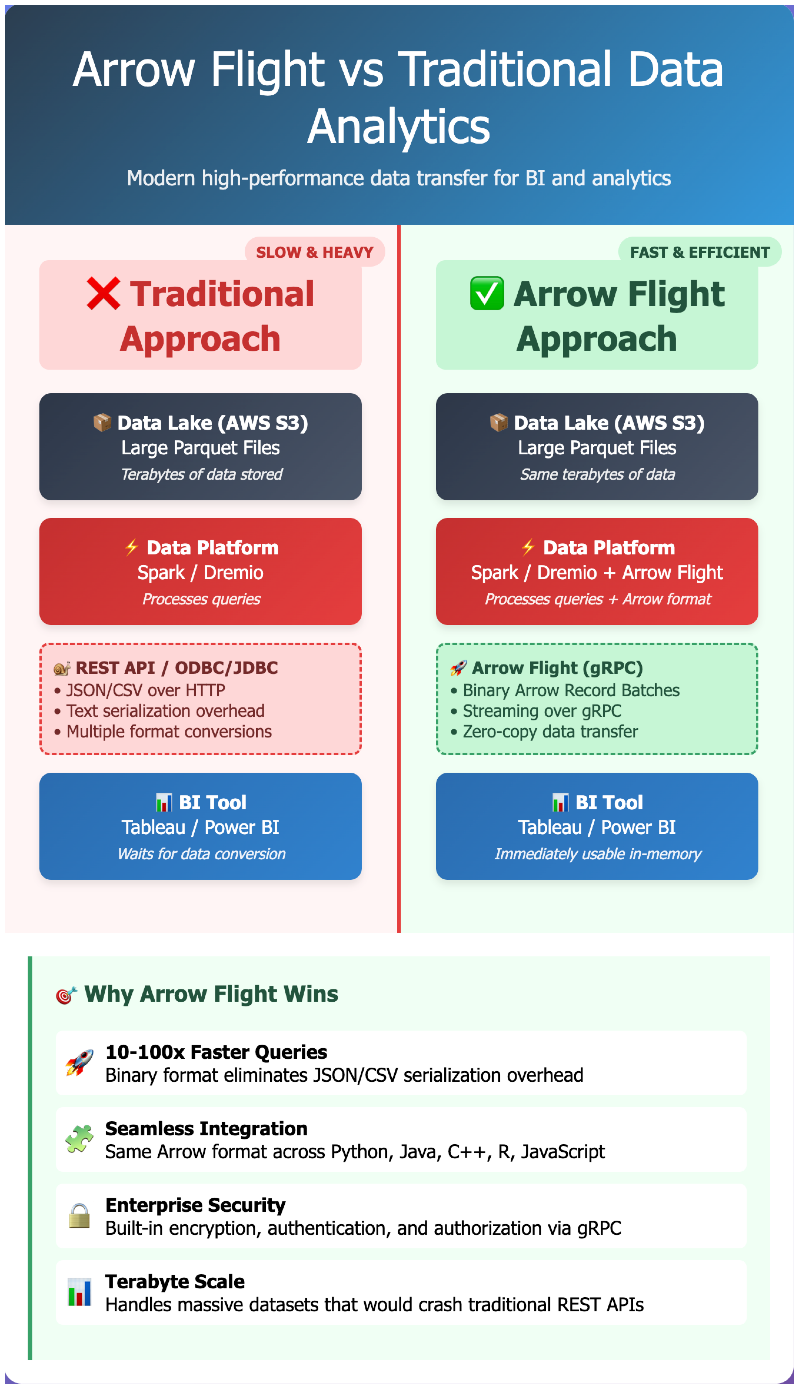
Arrow Flight SQL
- Adds SQL support on top of Arrow Flight.
- Submit SQL queries to a server and receive Arrow Flight responses.
- Easier for BI tools (e.g. Tableau, Power BI) connect to a Flight SQL server.
ADBC
ADBC stands for Arrow Database Connectivity. It’s a set of libraries and standards that define how to connect to databases using Apache Arrow data structures.
Think of it as a modern, Arrow-based alternative to ODBC/JDBC — but built for columnar analytics and big data workloads.
#dataformat #arrow #flightsql #flightrpc #adbc
[Avg. reading time: 3 minutes]
Delta
Delta Lake is an open-source storage layer that brings ACID transactions to Apache Spark and big data workloads. It sits on top of existing cloud storage systems like S3, ADLS, or GCS and adds transactional consistency and schema enforcement to your Parquet files.
Use Cases
Data Lakes with ACID Guarantees: Perfect for real-time and batch data processing in Data Lake environments.
Streaming + Batch Workflows: Unified processing with support for incremental updates.
Time Travel: Easy rollback and audit of data versions.
Upserts (MERGE INTO): Efficient updates/deletes on Parquet data using Spark SQL.
Slowly Changing Dimensions (SCD): Managing dimension tables in a data warehouse setup.
Technical Context
Underlying Format: Parquet
Transaction Log: _delta_log folder with JSON commit files
Operations Supported:
-MERGE
-UPDATE / DELETE
-OPTIMIZE / ZORDER
Integration: Supported in open-source via delta-rs, [Delta Kernel], and Delta Standalone Reader.
git clone https://github.com/gchandra10/python_delta_demo
[Avg. reading time: 2 minutes]
Protocol
Protocols are standardized rules that govern how data is transmitted, formatted, and processed across systems.
In Big Data, protocols are essential for:
- Data ingestion (getting data in)
- Inter-node communication in clusters
- Remote access to APIs/services
- Serialization of structured data
- Security and authorization
| Protocol | Layer | Use Case Example |
|---|---|---|
| HTTP/HTTPS | Application | REST API for ingesting external data |
| Kafka | Messaging | Stream processing with Spark or Flink |
| gRPC | RPC | Microservices in ML model serving |
| MQTT | Messaging | IoT data push to cloud |
| Avro/Proto | Serialization | Binary data for logs and schema |
| OAuth/Kerberos | Security | Secure access to data lakes |
[Avg. reading time: 2 minutes]
HTTP
Basics
HTTP (HyperText Transfer Protocol) is the foundation of data communication on the web, used to transfer data (such as HTML files and images).
GET - Navigate to a URL or click a link in real life.
POST - Submit a form on a website, like a username and password.
Popular HTTP Status Codes
200 Series (Success): 200 OK, 201 Created.
300 Series (Redirection): 301 Moved Permanently, 302 Found.
400 Series (Client Error): 400 Bad Request, 401 Unauthorized, 404 Not Found.
500 Series (Server Error): 500 Internal Server Error, 503 Service Unavailable.
---
[Avg. reading time: 3 minutes]
Monolithic Architecture
Definition: A monolithic architecture is a software design pattern in which an application is built as a unified unit. All application components (user interface, business logic, and data access layers) are tightly coupled and run as a single service.
Characteristics: This architecture is simple to develop, test, deploy, and scale vertically. However, it can become complex and unwieldy as the application grows.

Examples
- Older/Traditional Banking Systems.
- Enterprise Resource Planning (SAP ERP) Systems.
- Content Management Systems like WordPress.
- Legacy Government Systems. (Tax filing, public records management, etc.)
Advantages and Disadvantages
Advantages: Simplicity in development and deployment, straightforward horizontal scaling, and often more accessible debugging since all components are in one place.
Disadvantages: Scaling challenges, difficulty implementing changes or updates (especially in large systems), and potential for more extended downtime during maintenance.
[Avg. reading time: 8 minutes]
Statefulness
The server stores information about the client’s current session in a stateful system. This is common in traditional web applications. Here’s what characterizes a stateful system:
Session Memory: The server remembers past interactions and may store session data like user authentication, preferences, and other activities.
Server Dependency: Since the server holds session data, the same server usually handles subsequent requests from the same client. This is important for consistency.
Resource Intensive: Maintaining state can be resource-intensive, as the server needs to manage and store session data for each client.
Example: A web application where a user logs in, and the server keeps track of their authentication status and interactions until they log out.
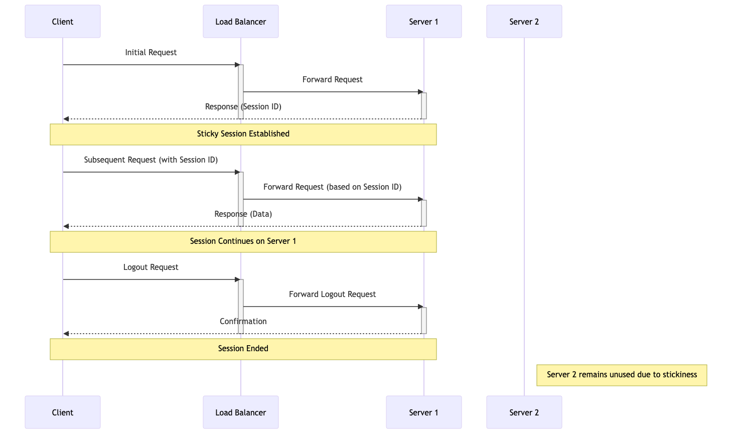
Diagram explaning Statefulness & Stickiness
In this diagram:
Initial Request: The client sends the initial request to the load balancer.
Load Balancer to Server 1: The load balancer forwards the request to Server 1.
Response with Session ID: Server 1 responds to the client with a session ID, establishing a sticky session.
Subsequent Requests: The client sends subsequent requests with the session ID.
Load Balancer Routes to Server 1: The load balancer forwards these requests to Server 1 based on the session ID, maintaining the sticky session.
Server 1 Processes Requests: Server 1 continues to handle requests from this client.
Server 2 Unused: Server 2 remains unused for this particular client due to the stickiness of the session with Server 1.
Stickiness (Sticky Sessions)
Stickiness or sticky sessions are used in stateful systems, particularly in load-balanced environments. It ensures that requests from a particular client are directed to the same server instance. This is important when:
Session Data: The server needs to maintain session data (like login status), and it’s stored locally on a specific server instance.
Load Balancers: In a load-balanced environment, without stickiness, a client’s requests could be routed to different servers, which might not have the client’s session data.
Trade-off: While it helps maintain session continuity, it can reduce the load balancing efficiency and might lead to uneven server load.
Methods of Implementing Stickiness
Cookie-Based Stickiness: The most common method, where the load balancer uses a special cookie to track the server assigned to a client.
IP-Based Stickiness: The load balancer routes requests based on the client’s IP address, sending requests from the same IP to the same server.
Custom Header or Parameter: Some load balancers can use custom headers or URL parameters to track and maintain session stickiness.
[Avg. reading time: 9 minutes]
Microservices
Microservices architecture is a method of developing software applications as a suite of small, independently deployable services. Each service in a microservices architecture is focused on a specific business capability, runs in its process, and communicates with other services through well-defined APIs. This approach stands in contrast to the traditional monolithic architecture, where all components of an application are tightly coupled and run as a single service.
Characteristics:
Modularity: The application is divided into smaller, manageable pieces (services), each responsible for a specific function or business capability.
Independence: Each microservice is independently deployable, scalable, and updatable. This allows for faster development cycles and easier maintenance.
Decentralized Control: Microservices promote decentralized data management and governance. Each service manages its data and logic.
Technology Diversity: Teams can choose the best technology stack for their microservice, leading to a heterogeneous technology environment.
Resilience: Failure in one microservice doesn’t necessarily bring down the entire application, enhancing the system’s overall resilience.
Scalability: Microservices can be scaled independently, allowing for more efficient resource utilization based on demand for specific application functions.
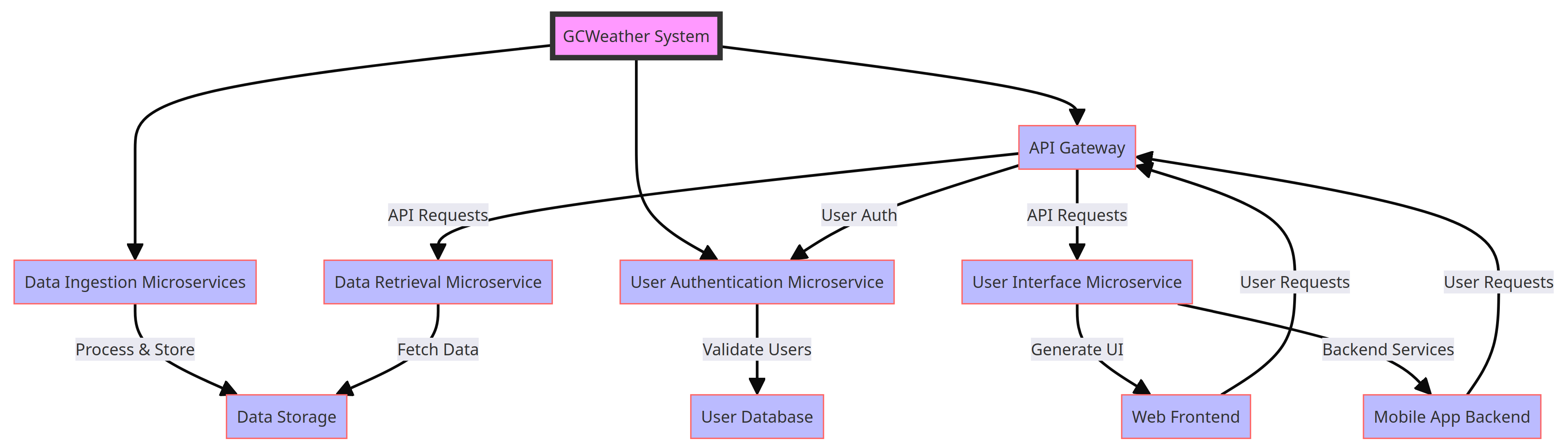
Sample architecture diagram of GCWeather System
Data Ingestion Microservices: Collect and process data from multiple sources.
Data Storage: Stores processed weather data and other relevant information.
User Authentication Microservice: Manages user authentication and communicates with the User Database for validation.
User Database: Stores user account information and preferences.
API Gateway: Central entry point for API requests, routes requests to appropriate microservices, and handles user authentication.
User Interface Microservice: Handles the logic for the user interface, serving web and mobile applications.
Data Retrieval Microservice: Fetches weather data from the Data Storage and provides it to the frontends.
Web Frontend: The web interface for end-users, making requests through the API Gateway.
Mobile App Backend: Backend services for the mobile application, also making requests through the API Gateway.
Advantages:
Agility and Speed: Smaller codebases and independent deployment cycles lead to quicker development and faster time-to-market.
Scalability: It is easier to scale specific application parts that require more resources.
Resilience: Isolated services reduce the risk of system-wide failures.
Flexibility in Technology Choices: Microservices can use different programming languages, databases, and software environments.
Disadvantages:
Complexity: Managing a system of many different services can be complex, especially regarding network communication, data consistency, and service discovery.
Overhead: Each microservice might need its own database and transaction management, leading to duplication and increased resource usage.
Testing Challenges: Testing inter-service interactions can be more complex compared to a monolithic architecture.
Deployment Challenges: Requires robust DevOps practices, including continuous integration and continuous deployment (CI/CD) pipelines.
[Avg. reading time: 6 minutes]
Statelessness
In a stateless system, each request from the client must contain all the information the server needs to fulfill that request. The server does not store any state of the client’s session. This is a crucial principle of RESTful APIs. Characteristics include:
No Session Memory: The server remembers nothing about the user once the transaction ends. Each request is independent.
Scalability: Stateless systems are generally more scalable because the server doesn’t need to maintain session information. Any server can handle any request.
Simplicity and Reliability: The stateless nature makes the system simpler and more reliable, as there’s less information to manage and synchronize across systems.
Example: An API where each request contains an authentication token and all necessary data, allowing any server instance to handle any request.
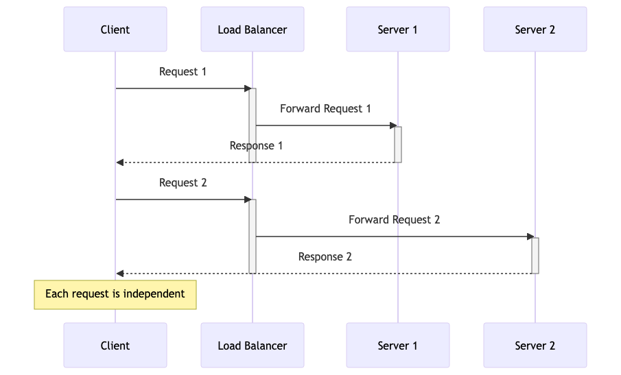
Diagram explaining Statelessness
In this diagram:
Request 1: The client sends a request to the load balancer.
Load Balancer to Server 1: The load balancer forwards Request 1 to Server 1.
Response from Server 1: Server 1 processes the request and sends a response back to the client.
Request 2: The client sends another request to the load balancer.
Load Balancer to Server 2: This time, the load balancer forwards Request 2 to Server 2.
Response from Server 2: Server 2 processes the request and responds to the client.
Statelessness: Each request is independent and does not rely on previous interactions. Different servers can handle other requests without needing a shared session state.
Token-Based Authentication
Common in stateless architectures, this method involves passing a token for authentication with each request instead of relying on server-stored session data. JWT (JSON Web Tokens) is a popular example.
[Avg. reading time: 1 minute]
Idempotency
Idempotency
This is a concept where an operation can be applied multiple times without changing the result beyond the initial application. It’s an essential concept in stateless architectures, especially for APIs.
[Avg. reading time: 9 minutes]
REST API
REpresentational State Transfer is a software architectural style developers apply to web APIs.
REST APIs provide simple, uniform interfaces because they can be used to make data, content, algorithms, media, and other digital resources available through web URLs. Essentially, REST APIs are the most common APIs used across the web today.
Use of a uniform interface (UI)
HTTP Methods
GET: This method allows the server to find the data you requested and send it back to you.
POST: This method permits the server to create a new entry in the database.
PUT: If you perform the ‘PUT’ request, the server will update an entry in the database.
DELETE: This method allows the server to delete an entry in the database.
Sample REST API
https://api.zippopotam.us/us/08028

http://api.tvmaze.com/search/shows?q=friends

https://jsonplaceholder.typicode.com/posts

https://jsonplaceholder.typicode.com/posts/1

https://jsonplaceholder.typicode.com/posts/1/comments

https://reqres.in/api/users?page=2

https://reqres.in/api/users/2
More examples
http://universities.hipolabs.com/search?country=United+States

https://itunes.apple.com/search?term=michael&limit=1000

https://www.boredapi.com/api/activity

https://techcrunch.com/wp-json/wp/v2/posts?per_page=100&context=embed
CURL
Install curl (Client URL)
curl is a CLI application available for all OS.
brew install curl
Usage
curl https://api.zippopotam.us/us/08028
curl https://api.zippopotam.us/us/08028 -o zipdata.json
Browser based
VS Code based
Summary
Definition: REST (Representational State Transfer) API is a set of guidelines for building web services. A RESTful API is an API that adheres to these guidelines and allows for interaction with RESTful web services.
How It Works: REST uses standard HTTP methods like GET, POST, PUT, DELETE, etc. It is stateless, meaning each request from a client to a server must contain all the information needed to understand and complete the request.
Data Format: REST APIs typically exchange data in JSON or XML format.
Purpose: REST APIs are designed to be a simple and standardized way for systems to communicate over the web. They enable the backend services to communicate with front-end applications (like SPAs) or other services.
Use Cases: REST APIs are used in web services, mobile applications, and IoT (Internet of Things) applications for various purposes like fetching data, sending commands, and more.
[Avg. reading time: 7 minutes]
API Performance
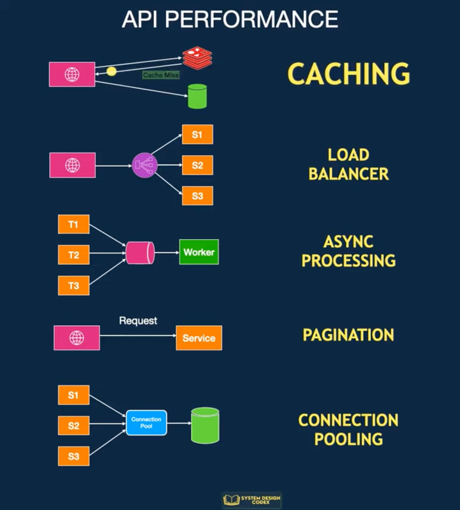
Src: systemdesigncodex.com
Caching
Store frequently accessed data in a cache so you can access it faster.
If there’s a cache miss, fetch the data from the database.
It’s pretty effective, but it can be challenging to invalidate and decide on the caching strategy.
Scale-out with Load Balancing
You can consider scaling your API to multiple servers if one server instance isn’t enough. Horizontal scaling is the way to achieve this.
The challenge will be to find a way to distribute requests between these multiple instances.
Load Balancing
It not only helps with performance but also makes your application more reliable.
However, load balancers work best when your application is stateless and easy to scale horizontally.
Pagination
If your API returns many records, you need to explore Pagination.
You limit the number of records per request.
This improves the response time of your API for the consumer.
Async Processing
With async processing, you can let the clients know that their requests are registered and under process.
Then, you process the requests individually and communicate the results to the client later.
This allows your application server to take a breather and give its best performance.
But of course, async processing may not be possible for every requirement.
Connection Pooling
An API often needs to connect to the database to fetch some data.
Creating a new connection for each request can degrade performance.
It’s a good idea to use connection pooling to set up a pool of database connections that can be reused across requests.
This is a subtle aspect, but connection pooling can dramatically impact performance in highly concurrent systems.
[Avg. reading time: 5 minutes]
API in Big Data World
Big data and REST APIs are often used together in modern data architectures. Here’s how they interact:
Data Ingestion: REST APIs can ingest data from various sources into big data platforms.
Data Access: REST APIs provide a convenient way for applications to query big data stores and receive responses in a usable format.
Microservices Architecture: In a microservices architecture, each microservice can handle some data processing and expose results through REST APIs.
Real-time Processing: REST APIs can serve real-time processed data from big data platforms to end-users or other systems.
Monitoring and Management: Big Data clusters and systems often come with management interfaces that expose REST APIs for monitoring, scaling, and managing resources.
Tool Ecosystem: Many Big Data tools and platforms, such as Hadoop, Spark, Kafka, and Elasticsearch, offer RESTful interfaces for managing and interacting with their services. Understanding these APIs is essential for working effectively with these tools.
Example of API
https://docs.redis.com/latest/rs/references/rest-api/
https://rapidapi.com/search/big-data
https://www.kaggle.com/discussions/general/315241
[Avg. reading time: 2 minutes]
Advance Python
- Environment
- Functional Programming Concepts
- Code Quality & Safety
- Decorator
- Serialization Deserialization
- Python Classes
- Unit Testing
- Data Frames
- Error Handling
- Logging]
- Flask
[Avg. reading time: 20 minutes]
Functional Programming Concepts
Functional programming in Python emphasizes the use of functions as first-class citizens, immutability, and declarative code that avoids changing state and mutable data.
def counter():
    count = 0  # Initialize the state
    count += 1
    return count

print(counter())
print(counter())
print(counter())
Regular functions internal State & mutable data
def counter():
    # Define an internal state using an attribute
    if not hasattr(counter, "count"):
        counter.count = 0  # Initialize the state

    # Modify the internal state
    counter.count += 1
    return counter.count

print(counter())
print(counter())
print(counter())
Internal state & immutability
Example without Lambda
increment = lambda x: x + 1

print(increment(5))  # Output: 6
print(increment(5))  # Output: 6
Using Lambda
Lambda functions as a way to write quick, one-off functions without defining a full function using def.
Example without Lambda
def square(x):
    return x ** 2

print(square(4))
Using Lambda
square = lambda x: x ** 2
print(square(4))
Without Lambda
def get_age(person):
    return person['age']

people = [
    {'name': 'Alice', 'age': 30},
    {'name': 'Bob', 'age': 25},
    {'name': 'Charlie', 'age': 35}
]

# Using a defined function to sort
sorted_people = sorted(people, key=get_age)
print(sorted_people)
Using Lambda
people = [
    {'name': 'Alice', 'age': 30},
    {'name': 'Bob', 'age': 25},
    {'name': 'Charlie', 'age': 35}
]

# Using a lambda function to sort
sorted_people = sorted(people, key=lambda person: person['age'])
print(sorted_people)
Map, Filter, Reduce Functions
Map, filter, and reduce are higher-order functions in Python that enable a functional programming style, allowing you to work with data collections in a more expressive and declarative manner.
Map
The map() function applies a given function to each item of an iterable (like a list or tuple) and returns an iterator with the results.
Map Without Functional Approach
numbers = [1, 2, 3, 4, 5]
squares = []
for num in numbers:
    squares.append(num ** 2)
print(squares)  # Output: [1, 4, 9, 16, 25]
Map With Lambda and Map
numbers = [1, 2, 3, 4, 5]
squares = list(map(lambda x: x ** 2, numbers))
print(squares)  # Output: [1, 4, 9, 16, 25]
Filter
The filter() function filters items out of an iterable based on whether they meet a condition defined by a function, returning an iterator with only those elements for which the function returns True.
Filter Without Functional Approach
numbers = [1, 2, 3, 4, 5]
evens = []
for num in numbers:
    if num % 2 == 0:
        evens.append(num)
print(evens)  # Output: [2, 4]
Filter using Functional Approach
numbers = [1, 2, 3, 4, 5]
evens = list(filter(lambda x: x % 2 == 0, numbers))
print(evens)  # Output: [2, 4]
Reduce
The reduce() function, from the functools module, applies a rolling computation to pairs of values in an iterable. It reduces the iterable to a single accumulated value.
At the same time, in many cases, simpler functions like sum() or loops may be more readable.
Reduce Without Functional Approach
- First, 1 * 2 = 2
- Then, 2 * 3 = 6
- Then, 6 * 4 = 24
- Then, 24 * 5 = 120
numbers = [1, 2, 3, 4, 5]
product = 1
for num in numbers:
    product *= num
print(product)  # Output: 120
Reduce With Lambda
from functools import reduce

numbers = [1, 2, 3, 4, 5]
product = reduce(lambda x, y: x * y, numbers)
print(product)  # Output: 120
Using an Initliazer
from functools import reduce

numbers = [1, 2, 3]

# Start with an initial value of 10
result = reduce(lambda x, y: x + y, numbers, 10)
print(result)
# Output: 16
Using SUM() instead of Reduce()
# So its not necessary to use Reduce all the time :)

numbers = [1, 2, 3, 4, 5]

# Using sum to sum the list
result = sum(numbers)
print(result)  # Output: 15
String Concatenation
from functools import reduce

words = ['Hello', 'World', 'from', 'Python']

result = reduce(lambda x, y: x + ' ' + y, words)
print(result)
# Output: "Hello World from Python"
List Comprehension and Generators
List Comprehension
List comprehension offers a shorter syntax when you want to create a new list based on the values of an existing list.
Generates the entire list in memory at once, which can consume a lot of memory for large datasets.
Uses: [ ]
Without List Comprehension
numbers = [1, 2, 3, 4, 5]
squares = []
for num in numbers:
    squares.append(num ** 2)
print(squares)
With List Comprehensions
numbers = [1, 2, 3, 4, 5]
squares = [x ** 2 for x in numbers]
print(squares)
List Generator
Generator expressions are used to create generators, which are iterators that generate values on the fly and yield one item at a time.
Generator expressions generate items lazily, meaning they yield one item at a time and only when needed. This makes them much more memory efficient for large datasets.
Uses: ( )
numbers = [1, 2, 3, 4, 5]
squares = (x ** 2 for x in numbers)
print(sum(squares))  # Output: 55
numbers = [1, 2, 3, 4, 5]
squares = (x ** 2 for x in numbers)
print(list(squares))
Best suited
- Only one line is in memory at a time.
- Suitable for processing large or infinite data streams.
#functional #lambda #generator #comprehension
[Avg. reading time: 8 minutes]
Code Quality & Safety
Type Hinting/Annotation
Type Hint
A type hint is a notation that suggests what type a variable, function parameter, or return value should be. It provides hints to developers and tools about the expected type but does not enforce them at runtime. Type hints can help catch type-related errors earlier through static analysis tools like mypy, and they enhance code readability and IDE support.
Type Annotation
Type annotation refers to the actual syntax used to provide these hints. It involves adding type information to variables, function parameters, and return types. Type annotations do not change how the code executes; they are purely for informational and tooling purposes.
Benefits
-
Improved Readability: Code with type annotations is easier to understand.
-
Tooling Support: IDEs can provide better autocompletion and error checking.
-
Static Analysis: Tools like mypy can check for type consistency, catching errors before runtime.
age: int = 25
name: str = "Rachel"
Here, age is annotated as an int, and name is annotated as a str.
Function Annotation
def add(x: int, y: int) -> int:
    return x + y
Complex Annotation
from typing import List, Dict

def get_user_info(user_ids: List[int]) -> Dict[int, str]:
    return {user_id: f"User {user_id}" for user_id in user_ids}
Secret Management
Simple way is to use Environment Variables.
Either create them in Shell or .env
Shell
export SECRET_KEY='your_secret_value'
Windows Users
Goto Environment Variables via GUI and create one.
pip install python-dotenv
Create a empty file .env
.env
SECRET_KEY=your_secret_key
DATABASE_URL=your_database_url
main.py
from dotenv import load_dotenv
import os

# Load environment variables from .env file
load_dotenv()

# Access the environment variables
secret_key = os.getenv("SECRET_KEY")
database_url = os.getenv("DATABASE_URL")

print(f"Secret Key: {secret_key}")
print(f"Database URL: {database_url}")
PDOC
Python Documentation
Docstring (Triple-quoted string)
def add(a: float, b: float) -> float:
    """
    Add two numbers.

    Args:
        a (float): The first number to add.
        b (float): The second number to add.

    Returns:
        float: The sum of the two numbers.

    Example:
        >>> add(2.5, 3.5)
        6.0
    """
    return a + b


def divide(a: float, b: float) -> float:
    """
    Divide one number by another.

    Args:
        a (float): The dividend.
        b (float): The divisor, must not be zero.

    Returns:
        float: The quotient of the division.

    Raises:
        ValueError: If the divisor (`b`) is zero.

    Example:
        >>> divide(10, 2)
        5.0
    """
    if b == 0:
        raise ValueError("The divisor (b) must not be zero.")
    return a / b
uv add pdoc

or

poetry add pdoc

or

pip install pdoc
poetry run pdoc filename.py -o ./docs

or

uv run pdoc filename.py -o ./docs
[Avg. reading time: 14 minutes]
Decorator
Decorators in Python are a powerful way to modify or extend the behavior of functions or methods without changing their code. Decorators are often used for tasks like logging, authentication, and adding additional functionality to functions. They are denoted by the “@” symbol and are applied above the function they decorate.
def say_hello():
    print("World")

say_hello()
How do we change the output without changing the say hello() function?
wrapper() is not reserved word. It can be anyting.
Use Decorators
# Define a decorator function
def hello_decorator(func):
    def wrapper():
        print("Hello,")
        func()  # Call the original function
    return wrapper

# Use the decorator to modify the behavior of say_hello
@hello_decorator
def say_hello():
    print("World")

# Call the decorated function
say_hello()
If you want to replace the new line character and the end of the print statement, use end=''
# Define a decorator function
def hello_decorator(func):
    def wrapper():
        print("Hello, ", end='')
        func()  # Call the original function
    return wrapper

# Use the decorator to modify the behavior of say_hello
@hello_decorator
def say_hello():
    print("World")

# Call the decorated function
say_hello()
Multiple functions inside the Decorator
def hello_decorator(func):
    def first_wrapper():
        print("First wrapper, doing something before the second wrapper.")
        #func()

    def second_wrapper():
        print("Second wrapper, doing something before the actual function.")
        #func()

    def main_wrapper():
        first_wrapper()  # Call the first wrapper
        second_wrapper()  # Then call the second wrapper, which calls the actual function
        func()

    return main_wrapper

@hello_decorator
def say_hello():
    print("World")

say_hello()
Args & Kwargs
*args: This is used to represent positional arguments. It collects all the positional arguments passed to the decorated function as a tuple.**kwargs: This is used to represent keyword arguments. It collects all the keyword arguments (arguments passed with names) as a dictionary.
from functools import wraps

def my_decorator(func):
    @wraps(func)
    def wrapper(*args, **kwargs):
        print("Positional Arguments (*args):", args)
        print("Keyword Arguments (**kwargs):", kwargs)
        result = func(*args, **kwargs)
        return result
    return wrapper

@my_decorator
def example_function(a, b, c=0, d=0):
    print("Function Body:", a, b, c, d)

# Calling the decorated function with different arguments
example_function(1, 2)
example_function(3, 4, c=5)
Popular Example
import time
from functools import wraps

def timer(func):
    @wraps(func)
    def wrapper(*args, **kwargs):
        start = time.time()
        result = func(*args, **kwargs)
        end = time.time()
        print(f"Execution time of {func.__name__}: {end - start} seconds")
        return result
    return wrapper

@timer
def add(x, y):
    """Returns the sum of x and y"""
    return x + y

@timer
def greet(name, message="Hello"):
    """Returns a greeting message with the name"""
    return f"{message}, {name}!"

print(add(2, 3))
print(greet("Rachel"))
The purpose of @wraps is to preserve the metadata of the original function being decorated.
Practice Item
from functools import wraps

# Decorator without @wraps
def decorator_without_wraps(func):
    def wrapper(*args, **kwargs):
        return func(*args, **kwargs)
    return wrapper

# Decorator with @wraps
def decorator_with_wraps(func):
    @wraps(func)
    def wrapper(*args, **kwargs):
        return func(*args, **kwargs)
    return wrapper

# Original function with a docstring
def original_function():
    """
    This is the original function's docstring.
    """
    pass

# Decorate the original function
decorated_function_without_wraps = decorator_without_wraps(original_function)
decorated_function_with_wraps = decorator_with_wraps(original_function)

# Display metadata of decorated functions
print("Without @wraps:")
print(f"Name: {decorated_function_without_wraps.__name__}")
print(f"Docstring: {decorated_function_without_wraps.__doc__}")

print("\nWith @wraps:")
print(f"Name: {decorated_function_with_wraps.__name__}")
print(f"Docstring: {decorated_function_with_wraps.__doc__}")
Memoization
Memoization is a technique used in Python to optimize the performance of functions by caching their results. When a function is called with a particular set of arguments, the result is stored. If the function is called again with the same arguments, the cached result is returned instead of recomputing it.
Benefits
Improves Performance: Reduces the number of computations by returning pre-computed results.
Efficient Resource Utilization: Saves computation time and resources, especially for recursive or computationally expensive functions.
git clone https://github.com/gchandra10/python_memoization
[Avg. reading time: 11 minutes]
Serialization-Deserialization
Serialization converts a data structure or object state into a format that can be stored or transmitted (e.g., file, message, or network).
Deserialization is the reverse process, reconstructing the original object from the serialized form.
(Python/Scala/Rust) Objects to JSON back to Objects (Python/Scala/Rust)
The analogy of translating from Spanish to English (Universal Language) and to German
JSON
JavaScript Object Notation (JSON)
A lightweight, human-readable, and machine-parsable text format.
Pros
- Easy to read and debug.
- Supported by almost all programming languages.
- Ideal for APIs and configuration files.
Cons
- Text-based -> larger size on disk.
- No native schema enforcement.
import json

# Serialization
data = {"name": "Alice", "age": 25, "city": "New York"}
json_str = json.dumps(data)
print(json_str)

# Deserialization
obj = json.loads(json_str)
print(obj["name"])
AVRO
Apache Avro is a binary serialization format designed for efficiency, compactness, and schema evolution.
- Compact & Efficient: Binary encoding → smaller and faster than JSON.
- Schema Evolution: Supports backward/forward compatibility.
- Rich Data Types: Handles nested, array, map, union types.
- Language Independent: Works across Python, Java, Scala, Rust, etc.
- Big Data Integration: Works seamlessly with Hadoop, Kafka, Spark.
- Self-Describing: Schema travels with the data.
Schemas
An Avro schema defines the structure of the Avro data format. It’s a JSON document that describes your data types and protocols, ensuring that even complex data structures are adequately represented. The schema is crucial for data serialization and deserialization, allowing systems to interpret the data correctly.
Example of Avro Schema
{
  "type": "record",
  "name": "Person",
  "namespace": "com.example",
  "fields": [
    {"name": "firstName", "type": "string"},
    {"name": "lastName", "type": "string"},
    {"name": "age", "type": "int"},
    {"name": "email", "type": ["null", "string"], "default": null}
  ]
}
Here is the list of Primitive & Complex Data Types which Avro supports:
- null,boolean,int,long,float,double,bytes,string
- records,enums,arrays,maps,unions,fixed
JSON vs Avro
| Feature | JSON | Avro |
|---|---|---|
| Format Type | Text-based (human-readable) | Binary (machine-efficient) |
| Size | Larger (verbose) | Smaller (compact) |
| Speed | Slower to serialize/deserialize | Much faster (binary encoding) |
| Schema | Optional / loosely defined | Mandatory and embedded with data |
| Schema Evolution | Not supported | Fully supported (backward & forward compatible) |
| Data Types | Basic (string, number, bool, array, object) | Rich (records, enums, arrays, maps, unions, fixed) |
| Readability | Human-friendly | Not human-readable |
| Integration | Common in APIs, configs | Common in Big Data (Kafka, Spark) |
| Use Case | Simple data exchange (REST APIs) | High-performance data pipelines, streaming systems |
In short,
- Use JSON when simplicity & readability matter.
- Use Avro when performance, compactness, and schema evolution matter (especially in Big Data systems).
git clone https://github.com/gchandra10/python_serialization_deserialization_examples.git
Parquet vs Avro
| Feature | Avro | Parquet |
|---|---|---|
| Format Type | Row-based binary format | Columnar binary format |
| Best For | Streaming, message passing, row-oriented reads/writes | Analytics, queries, column-oriented reads |
| Compression | Moderate (row blocks) | Very high (per column) |
| Read Pattern | Reads entire rows | Reads only required columns → faster for queries |
| Write Pattern | Fast row inserts / appends | Best for batch writes (not streaming-friendly) |
| Schema | Embedded JSON schema, supports evolution | Embedded schema, supports evolution (with constraints) |
| Data Evolution | Flexible backward/forward compatibility | Supported, but limited (column addition/removal) |
| Use Case | Kafka, Spark streaming, data ingestion pipelines | Data warehouses, lakehouse tables, analytics queries |
| Integration | Hadoop, Kafka, Spark, Hive | Spark, Hive, Trino, Databricks, Snowflake |
| Readability | Not human-readable | Not human-readable |
| Typical File Extension | .avro | .parquet |
#serialization #deserialization #avro
[Avg. reading time: 5 minutes]
Python Classes
Classes are templates used to define the properties and methods of objects in code. They can describe the kinds of data the class holds and how a programmer interacts with them.
Attributes - Properties
Methods - Action
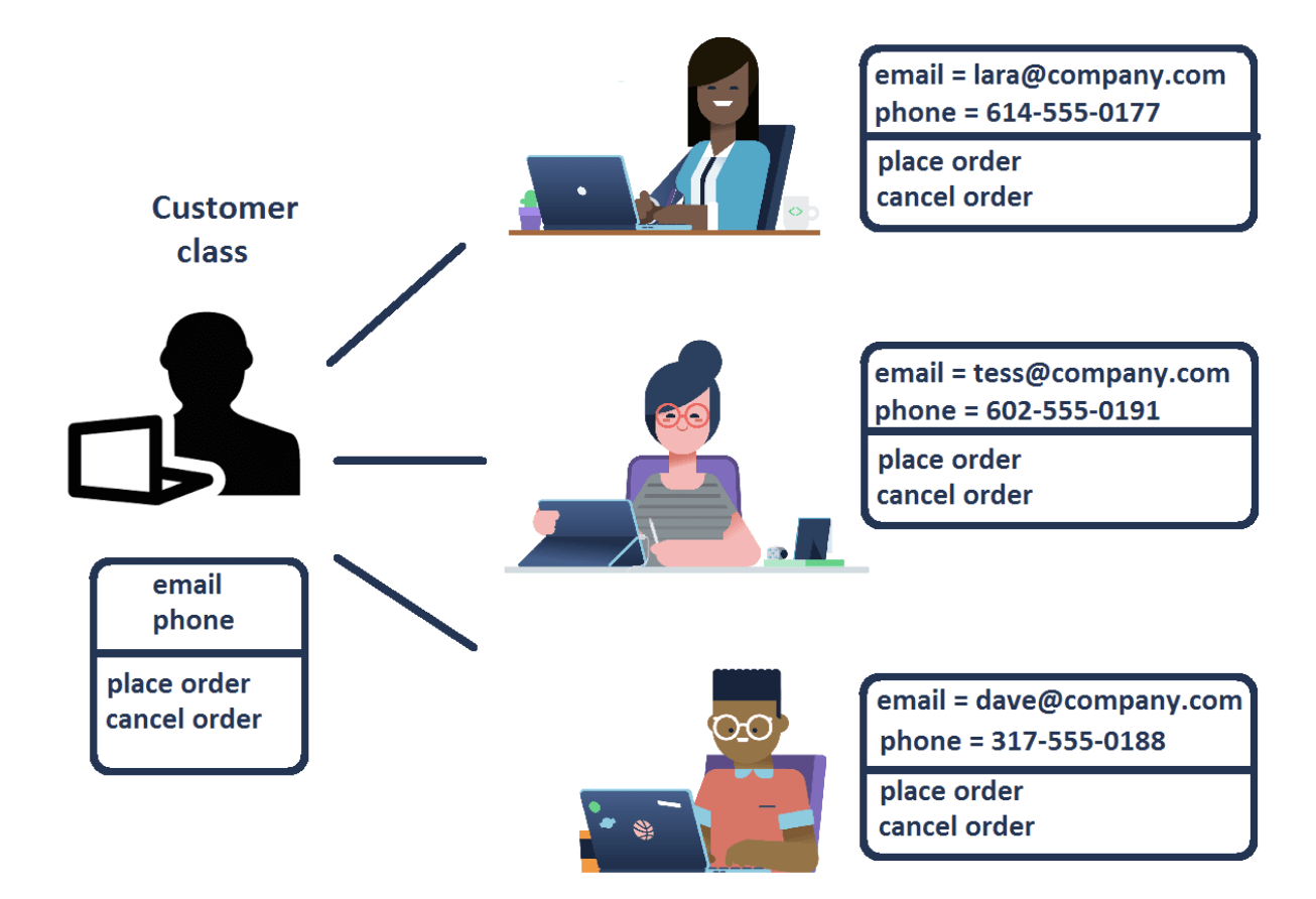
Img src: https://www.datacamp.com/tutorial/python-classes
class Dog:
    def __init__(self, name, age):
        self.name = name
        self.age = age

    def bark(self):
        print(f"{self.name} says woof! and its {self.age} years old")

my_dog = Dog("Buddy", 2)

my_dog.bark()
Class Definition: We start with the class keyword followed by Dog, the name of our class. This is the blueprint for creating Dog objects.
Constructor Method (__init__): This particular method is called automatically when a new Dog object is created. It initializes the object’s attributes. In this case, each Dog has a name and an age. The self parameter is a reference to the current instance of the class.
Attribute: self.name and self.age These are attributes of the class. These variables are associated with each class instance, holding the specific data.
Method: bark It is a method of the class. It’s a function that all Dog instances can perform. When called, it prints a message indicating that the dog is barking.
Python supports two types of methods within classes.
- StaticMethod
- InstanceMethod
Fork & Clone
git clone https://github.com/gchandra10/python_classes_demo.git
[Avg. reading time: 3 minutes]
Unit Testing
A unit test tests a small “unit” of code - usually a function or method - independently from the rest of the program.
Some key advantages of unit testing include:
- Isolates code - This allows testing individual units in isolation from other parts of the codebase, making bugs easier to identify.
- Early detection - Tests can catch issues early in development before code is deployed, saving time and money.
- Regression prevention - Existing unit tests can be run whenever code is changed to prevent new bugs or regressions.
- Facilitates changes - Unit tests give developers the confidence to refactor or update code without breaking functionality.
- Quality assurance - High unit test coverage helps enforce quality standards and identify edge cases.
Every language has its unit testing framework. In Python, some popular ones are
- unittest
- pytest
- doctest
- testify
Example:
Using Pytest & UV
git clone https://github.com/gchandra10/pytest-demo.git
Using Unittest & Poetry
git clone https://github.com/gchandra10/python_calc_unittests
[Avg. reading time: 19 minutes]
Data Frames
DataFrames are the core abstraction for tabular data in modern data processing — used across analytics, ML, and ETL workflows.
They provide:
- Rows and columns like a database table or Excel sheet.
- Rich APIs to filter, aggregate, join, and transform data.
- Interoperability with CSV, Parquet, JSON, and Arrow.
Pandas
Pandas is a popular Python library for data manipulation and analysis. A DataFrame in Pandas is a two-dimensional, size-mutable, and heterogeneous tabular data structure with labeled axes (rows and columns).
Eager Evaluation: Pandas performs operations eagerly, meaning that each operation is executed immediately when called.
In-Memory Copy - Full DataFrame in RAM, single copy
Sequential Processing - Single threaded, one operation at at time.
Pros
- Easy to use and intuitive syntax.
- Rich functionality for data manipulation, including filtering, grouping, and merging.
- Large ecosystem and community support.
Cons
- Performance issues with very large datasets (limited by memory).
- Single-threaded operations, making it slower for big data tasks.
Example
import pandas as pd

# Load the CSV file using Pandas
df = pd.read_csv('data/sales_100.csv')

# Display the first few rows
print(df.head())
Polars
Polars is a fast, multi-threaded DataFrame library in Rust and Python, designed for performance and scalability. It is known for its efficient handling of larger-than-memory datasets.
Supports both eager and lazy evaluation.
Lazy Evaluation: Instead of loading the entire CSV file into memory right away, a Lazy DataFrame builds a blueprint or execution plan describing how the data should be read and processed. The actual data is loaded only when the computation is triggered (for example, when you call a collect or execute command).
Optimizations: Using scan_csv allows Polars to optimize the entire query pipeline before loading any data. This approach is beneficial for large datasets because it minimizes memory usage and improves execution efficiency.
- pl.read_csv() or pl.read_parquet() - eager evaluation
- pl.scan_csv() or pl.scan_parquet() - lazy evaluation
Parallel Execution: Multi-threaded compute.
Columnar efficiency: Uses Arrow columnar memory format under the hood.
Pros
- High performance due to multi-threading and memory-efficient execution.
- Lazy evaluation, optimizing the execution of queries.
- Handles larger datasets effectively.
Cons
- Smaller community and ecosystem compared to Pandas.
- Less mature with fewer third-party integrations.
Example
import polars as pl

# Load the CSV file using Polars
df = pl.scan_csv('data/sales_100.csv')

print(df.head())

# Display the first few rows
print(df.collect())

df1 = pl.read_csv('data/sales_100.csv')
print(df1.head())
Dask
Dask is a parallel computing library that scales Python libraries like Pandas for large, distributed datasets.
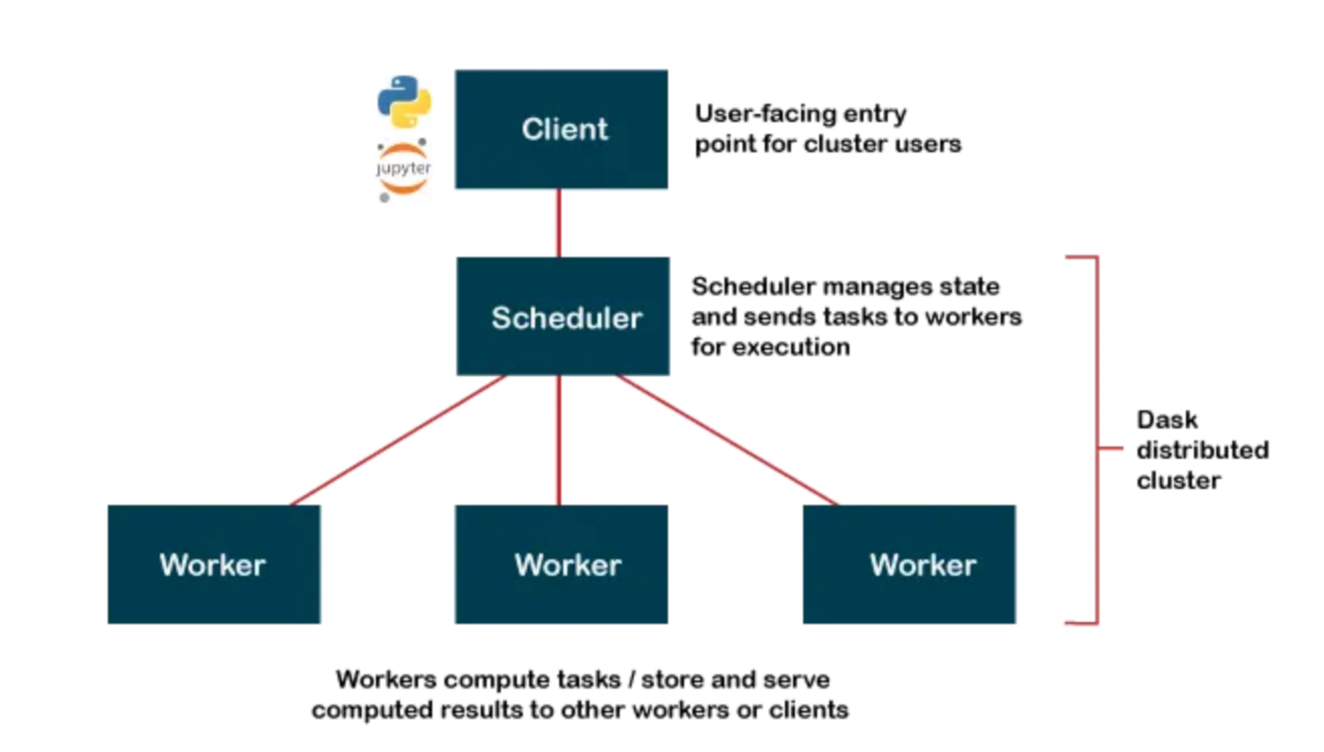
Client (Python Code)
   │
   ▼
Scheduler (builds + manages task graph)
   │
   ▼
Workers (execute tasks in parallel)
   │
   ▼
Results gathered back to client
Open Source https://docs.dask.org/en/stable/install.html
Dask Cloud Coiled Cloud
Lazy Reading: Dask builds a task graph instead of executing immediately — computations run only when triggered (similar to Polars lazy execution).
Partitioning: A Dask DataFrame is split into many smaller Pandas DataFrames (partitions) that can be processed in parallel.
Task Graph: Dask represents your workflow as a directed acyclic graph (DAG) showing the sequence and dependencies of tasks.
Distributed Compute: Dask executes tasks across multiple cores or machines, enabling scalable, parallel data processing.
import dask.dataframe as dd

ddf = dd.read_csv(
    "data/sales_*.csv",
    dtype={"category": "string", "value": "float64"},
    blocksize="64MB"
)

# 2) Lazy transform: per-partition groupby + sum, then global combine
agg = ddf.groupby("category")["value"].sum().sort_values(ascending=False)

# 3) Trigger execution and bring small result to driver
result = agg.compute()

print(result.head(10))
blocksize determines the parition. If omitted dask automatically uses 64MB
flowchart LR
  A1[CSV part 1] --> P1[parse p1]
  A2[CSV part 2] --> P2[parse p2]
  A3[CSV part 3] --> P3[parse p3]

  P1 --> G1[local groupby-sum p1]
  P2 --> G2[local groupby-sum p2]
  P3 --> G3[local groupby-sum p3]

  G1 --> C[combine-aggregate]
  G2 --> C
  G3 --> C

  C --> S[sort values]
  S --> R[collect to Pandas]
Pros
- Can handle datasets that don’t fit into memory by processing in parallel.
- Scales to multiple cores and clusters, making it suitable for big data tasks.
- Integrates well with Pandas and other Python libraries.
Cons
- Slightly more complex API compared to Pandas.
- Performance tuning can be more challenging.
Where to start?
- Start with Pandas for learning and small datasets.
- Switch to Polars when performance matters.
- Use Dask when data exceeds single-machine memory or needs cluster execution.
git clone https://github.com/gchandra10/python_dataframe_examples.git
Pandas vs Polars vs Dask
| Feature | Pandas | Polars | Dask |
|---|---|---|---|
| Language | Python | Rust with Python bindings | Python |
| Execution Model | Single-threaded | Multi-threaded | Multi-threaded, distributed |
| Data Handling | In-memory | In-memory, Arrow-based | In-memory, out-of-core |
| Scalability | Limited by memory | Limited to single machine | Scales across clusters |
| Performance | Good for small to medium data | High performance for single machine | Good for large datasets |
| API Familiarity | Widely known, mature | Similar to Pandas | Similar to Pandas |
| Ease of Use | Very easy, large ecosystem | Easy, but smaller ecosystem | Moderate, requires understanding of parallelism |
| Fault Tolerance | None | Limited | High, with task retries and rescheduling |
| Machine Learning | Integration with Python ML libs | Preprocessing only | Integration with Dask-ML and other libs |
| Lazy Evaluation | No | Yes | Yes, with task graphs |
| Best For | Data analysis, small datasets | Fast preprocessing on single machine | Large-scale data processing |
| Cluster Management | N/A | N/A | Supports Kubernetes, YARN, etc. |
| Use Cases | Data manipulation, analysis | Fast data manipulation | Large data, ETL, scaling Python code |
[Avg. reading time: 8 minutes]
Error Handling
Python uses try/except blocks for error handling.
The basic structure is:
try:
    # Code that may raise an exception
except ExceptionType:
    # Code to handle the exception
finally:
    # Code executes all the time
Uses
Improved User Experience: Instead of the program crashing, you can provide a user-friendly error message.
Debugging: Capturing exceptions can help you log errors and understand what went wrong.
Program Continuity: Allows the program to continue running or perform cleanup operations before terminating.
Guaranteed Cleanup: Ensures that certain operations, like closing files or releasing resources, are always performed.
Some key points
-
You can catch specific exception types or use a bare except to catch any exception.
-
Multiple except blocks can be used to handle different exceptions.
-
An else clause can be added to run if no exception occurs.
-
A finally clause will always execute, whether an exception occurred or not.
Without Try/Except
x = 10 / 0
Basic Try/Except
try:
    x = 10 / 0
except ZeroDivisionError:
    print("Error: Division by zero!")
Generic Exception
try:
    file = open("nonexistent_file.txt", "r")
except:
    print("An error occurred!")
Find the exact error
try:
    file = open("nonexistent_file.txt", "r")
except Exception as e:
    print(str(e))
Raise - Else and Finally
try:
    x = -10
    if x <= 0:
        raise ValueError("Number must be positive")
except ValueError as ve:
    print(f"Error: {ve}")
else:
    print(f"You entered: {x}")
finally:
    print("This will always execute")
try:
    x = 10
    if x <= 0:
        raise ValueError("Number must be positive")
except ValueError as ve:
    print(f"Error: {ve}")
else:
    print(f"You entered: {x}")
finally:
    print("This will always execute")
Nested Functions
def divide(a, b):
    try:
        result = a / b
        return result
    except ZeroDivisionError:
        print("Error in divide(): Cannot divide by zero!")
        raise  # Re-raise the exception

def calculate_and_print(x, y):
    try:
        result = divide(x, y)
        print(f"The result of {x} divided by {y} is: {result}")
    except ZeroDivisionError as e:
        print(str(e))
    except TypeError as e:
        print(str(e))

# Test the nested error handling
print("Example 1: Valid division")
calculate_and_print(10, 2)

print("\nExample 2: Division by zero")
calculate_and_print(10, 0)

print("\nExample 3: Invalid type")
calculate_and_print("10", 2)
#errorhandling #exception #try
[Avg. reading time: 7 minutes]
Logging
Python’s logging module provides a flexible framework for tracking events in your applications. It’s used to log messages to various outputs (console, files, etc.) with different severity levels like DEBUG, INFO, WARNING, ERROR, and CRITICAL.
Use Cases of Logging
Debugging: Identify issues during development. Monitoring: Track events in production to monitor behavior. Audit Trails: Capture what has been executed for security or compliance. Error Tracking: Store errors for post-mortem analysis. Rotating Log Files: Prevent logs from growing indefinitely using size or time-based rotation.
Python Logging Levels
| Level | Usage | Numeric Value | Description |
|---|---|---|---|
DEBUG | Detailed information for diagnosing problems. | 10 | Useful during development and debugging stages. |
INFO | General information about program execution. | 20 | Highlights normal, expected behavior (e.g., program start, process completion). |
WARNING | Indicates something unexpected but not critical. | 30 | Warns of potential problems or events to monitor (e.g., deprecated functions, nearing limits). |
ERROR | An error occurred that prevented some part of the program from working. | 40 | Represents recoverable errors that might still allow the program to continue running. |
CRITICAL | Severe errors indicating a major failure. | 50 | Marks critical issues requiring immediate attention (e.g., system crash, data corruption). |
INFO
import logging

logging.basicConfig(level=logging.INFO)  # Set the logging level to INFO

logging.debug("This is a debug message.")
logging.info("This is an info message.")
logging.warning("This is a warning message.")
logging.error("This is an error message.")
logging.critical("This is a critical message.")
Error
import logging

logging.basicConfig(level=logging.ERROR)  # Set the logging level to ERROR

logging.debug("This is a debug message.")
logging.info("This is an info message.")
logging.warning("This is a warning message.")
logging.error("This is an error message.")
logging.critical("This is a critical message.")
import logging

logging.basicConfig(
    level=logging.DEBUG,
    format = '%(asctime)s - %(name)s - %(levelname)s - %(message)s'
)

logging.debug("This is a debug message.")
logging.info("This is an info message.")
logging.warning("This is a warning message.")
More Examples
git clone https://github.com/gchandra10/python_logging_examples.git
[Avg. reading time: 1 minute]
Flask Demo
- Setup
- Flask Demo
- Flask Demo-01
- Flask Demo-02
- Flask Demo-03
- Flask Demo-04
- Flask Demo-05
- API Testing
- Flask Demo Testing
[Avg. reading time: 4 minutes]
Setup
Libraries used in Poetry/UV
poetry add flask
poetry add redis
poetry add python-dotenv
poetry add flask-httpauth
poetry add flask-jwt-extended
poetry add flask-restful
poetry add flask-restx
poetry add pyarrow
poetry add pyjwt
poetry add pymysql
poetry add pyyaml
poetry add black
or
uv add flask
uv add redis
uv add python-dotenv
uv add flask-httpauth
uv add flask-jwt-extended
uv add flask-restful
uv add flask-restx
uv add pyarrow
uv add pyjwt
uv add pymysql
uv add pyyaml
uv add black
Install VSCode https://code.visualstudio.com/
(not Visual Studio)
Install the following Extensions
-
Thunder Client (https://marketplace.visualstudio.com/items?itemName=rangav.vscode-thunder-client)
-
MySQL (https://marketplace.visualstudio.com/items?itemName=cweijan.vscode-mysql-client2)
Optional Items
Always Data (FREE)
https://www.alwaysdata.com/en/
Upstash (FREE)
#api #flask #mysqlcloud #upstash
[Avg. reading time: 5 minutes]
Flask Demo
Clone this Repo from your laptops.
https://github.com/gchandra10/python_flask_demo.git
If you don’t have GIT installed, follow these steps. If you already have it, skip to the cloning part
For Both Windows and Mac:
-
Install Git:
- Windows: Download and install Git from git-scm.com
- Mac: Install Git using Homebrew by typing
brew install gitin the Terminal. If you don’t have Homebrew, you can download Git from git-scm.com.
-
Open Terminal or Command Prompt:
- Windows: Open Command Prompt (search for ‘cmd’ in the Start menu).
- Mac: Open Terminal (you can find it using Spotlight with
Cmd + Spaceand then type “Terminal”).
-
Check Git Installation: You can check if Git is installed by typing
git --versionin your Command Prompt or Terminal. -
Navigate to the Directory where you want the cloned repository:
- Use the
cdcommand to change directories. For example,cd Documents/Projects.
- Use the
-
Clone the Repository:
- Use the command
git clone [URL]. - Replace
[URL]with the URL of the Git repository you want to clone. You can get this URL by going to the repository page on GitHub (or another Git hosting service) and clicking the “Clone or download” button.
- Use the command
Example:
git clone https://github.com/gchandra10/python_flask_demo.git
[Avg. reading time: 1 minute]
Flask Demo - 01
Run the script
uv run python api_demo/flask_01_simple_app.py

or

poetry run python api_demo/flask_01_simple_app.py
Open the browser and visit http://127.0.0.1:5001
@app, @api, and @auth are decorators specific to Flask and Flask-RESTful libraries. They are used to define routes, API endpoints, and authentication rules.
[Avg. reading time: 2 minutes]
Flask Demo - 02
CRUD stands for Create, Read, Update, and Delete. These are the four basic operations of persistent storage in software development.
uv run python api_demo/flask_02_crud_app.py

or

poetry run python api_demo/flask_02_crud_app.py
Create a new Item
curl -X POST -H "Content-Type: application/json" -d '{"name":"item 99"}' http://127.0.0.1:5002/items
Update Existing Item
curl -X PUT -H "Content-Type: application/json" -d '{"id":3,"name":"item 3"}' http://127.0.0.1:5002/items/3
Delete Existing Item
curl -X DELETE http://127.0.0.1:5002/items/3
#flask #python #git #api #crud
[Avg. reading time: 8 minutes]
Flask Demo - 03
HTTP Basic Authentication
-
Simplicity: Basic Authentication is simple to implement, as it doesn’t require additional libraries or infrastructure. It’s part of the HTTP standard.
-
Suitability for Simple Use Cases: It’s suitable for simple, internal applications or services where ease of implementation is more critical than advanced security features.
-
Limited Security: The credentials are only base64 encoded, not encrypted, making it less secure unless used with HTTPS. It’s also more vulnerable to CSRF (Cross-Site Request Forgery) attacks.
-
Stateful: Basic Authentication is typically stateful, requiring the server to maintain session state, which can be a drawback in distributed systems.
uv run python api_demo/flask_03_basic_auth_app.py

or

poetry run python api_demo/flask_03_basic_auth_app.py
http://127.0.0.1:5003/items
Other @auth decorators
@auth.verify_password:
This decorator defines a function that verifies user credentials during authentication.
Example:
@auth.verify_password
def verify_password(username, password):
    # Check username and password, return username if authentication succeeds
auth.username():
-
After successful authentication, you can use
auth.username()to retrieve the authenticated username within a route function. -
Example:
@app.route('/profile')
@auth.login_required
def get_profile():
    username = auth.username()
    # Use the username to fetch user-specific data
@auth.login_required:
-
This decorator protects routes that require authentication. It ensures that only authenticated users can access the decorated route.
-
Example:
@app.route('/secure_data')
@auth.login_required
def secure_data():
    # Only authenticated users can access this route
@auth.error_handler:
-
You can define a custom error handler for authentication failures using this decorator. It allows you to handle authentication errors in a customized way.
-
Example:
@auth.error_handler
def unauthorized():
    return jsonify({"message": "Unauthorized access"}), 401
@auth.token_authentication:
-
If you want to implement token-based authentication, you can use this decorator to specify a function that verifies tokens.
-
Example:
@auth.token_authentication
def verify_token(token):
    # Check if the token is valid and return the associated user
@auth.get_password and @auth.get_user_roles:
-
These decorators allow you to customize how passwords and user roles are retrieved from your data source. They are useful for complex authentication systems.
-
Example:
@auth.get_password
def get_password(username):
    # Retrieve and return the password for the given username
Usage
users = {
    "user1": "password1",
    "user2": "password2"
}

user_roles = {
    "user1": ["admin"],
    "user2": ["user"]
}

@auth.get_password
def get_password(username):
    return users.get(username)

@auth.get_user_roles
def get_user_roles(user):
    return user_roles.get(user)

tokens = {
    "token1": "user1",
    "token2": "user2"
}

@auth.verify_token
def verify_token(token):
    if token in tokens:
        return tokens[token]
#flask #python #git #api #authentication
[Avg. reading time: 9 minutes]
Flask Demo - 04
JWT (JSON Web Tokens)
JWT (JSON Web Tokens) offers a secure way to transmit information between parties as a JSON object. It provides several advantages over traditional username/password authentication, especially in stateless applications. However, it’s essential to understand that JWT is not just about authentication; it’s also about information exchange and maintaining stateless sessions. Here’s a breakdown of its security aspects and how it compares to traditional methods:
-
Statelessness and Scalability: JWTs are self-contained and carry all the necessary information within the token. This stateless nature allows for better scalability, as the server does not need to maintain a session state.
-
Flexibility: JWTs can be used across different domains, making them ideal for microservices architecture and authenticating API requests in a distributed system.
-
Security: JWTs support more robust and flexible cryptographic algorithms than Basic Authentication. They can be signed and optionally encrypted.
-
Compact and Self-Contained: JWTs contain all the required information about the user, avoiding the need to query the database more than once. This can improve performance by reducing the need for repeated database lookups.
-
Rich Payload: JWTs can contain a payload of claims. These claims can include user details and permissions applicable for fine-grained access control in APIs.
-
Widely Supported: JWTs are widely supported across various programming languages and platforms.
-
Use in Modern Authentication Flows: JWTs are commonly used in OAuth 2.0 and OpenID Connect flows, standard authentication and authorization protocols used by many modern applications.
However, JWTs are not without their drawbacks and must be used correctly to ensure security:
-
Storage: Tokens are typically stored in client-side storage, which can be vulnerable to XSS attacks. Proper precautions must be taken to mitigate this risk.
-
No Server-Side Revocation: Since JWTs are stateless, once a token is issued, it cannot be revoked before it expires. This can be a problem if a token is compromised.
-
Sensitive Data: Don’t store sensitive data in a JWT. Although it’s encoded, it’s not encrypted. Anyone who intercepts the token can decode it and read its contents.
-
Transmission Security: Always use HTTPS to transmit JWTs to prevent man-in-the-middle attacks.
Java Web Tokens
uv run python api_demo/flask_04_jwt_auth_app.py

or

poetry run python api_demo/flask_04_jwt_auth_app.py
curl -X POST -H "Content-Type: application/json" -d '{"username":"user1", "password":"password1"}' http://127.0.0.1:5004/login

The token expires in 30 seconds.

curl -X GET -H "Authorization: Bearer eyJhbGciOiJIUzI1NiIsInR5cCI6IkpXVCJ9.eyJmcmVzaCI6ZmFsc2UsImlhdCI6MTcwMzUzMzIwNiwianRpIjoiMGY5MmNlNTUtNmRmNS00YjM0LTkyMWQtMDc3NGU5YzhkMmY3IiwidHlwZSI6ImFjY2VzcyIsInN1YiI6InVzZXIxIiwibmJmIjoxNzAzNTMzMjA2LCJjc3JmIjoiZTBmMDg3MmMtZWQ2ZC00MTdhLTg1NDYtMDA1NWMxOTIzZjkzIiwiZXhwIjoxNzAzNTMzMjM2fQ.dfkiOYI2ka00pYvRQ316lt4kESEGN7ZerE9Q2q75XQM"
http://127.0.0.1:5004/items
Why is JWT popular? YT Video
https://www.youtube.com/watch?v=P2CPd9ynFLg&ab_channel=ByteByteGo
[Avg. reading time: 3 minutes]
Flask Demo - 05
Flask-RESTX is an extension of Flask that helps you quickly build RESTful APIs with features like input validation, API documentation, and request/response parsing — all with minimal boilerplate.
It’s a community-maintained fork of the now-inactive Flask-RESTPlus project.
Flask by itself is a lightweight web framework — it doesn’t give you:
- Automatic request parsing
- Swagger/OpenAPI documentation
- Input validation
- Namespacing for large APIs
Flask-RESTX adds all that.
Remember to update config.yaml with your credentials
Get sakila-data-02.sql and sakila-schema-01.sql from here.
https://github.com/gchandra10/sakila\_schema\_data\_mysql
Use MySQL Workbench Load sakila-schema-01.sql first followed by
sakila-data-02.sql
uv run python api_demo/flask_06_mysql_app.py

or

poetry run python api_demo/flask_06_mysql_app.py
#flask #python #git #api #mysql
[Avg. reading time: 5 minutes]
API Testing
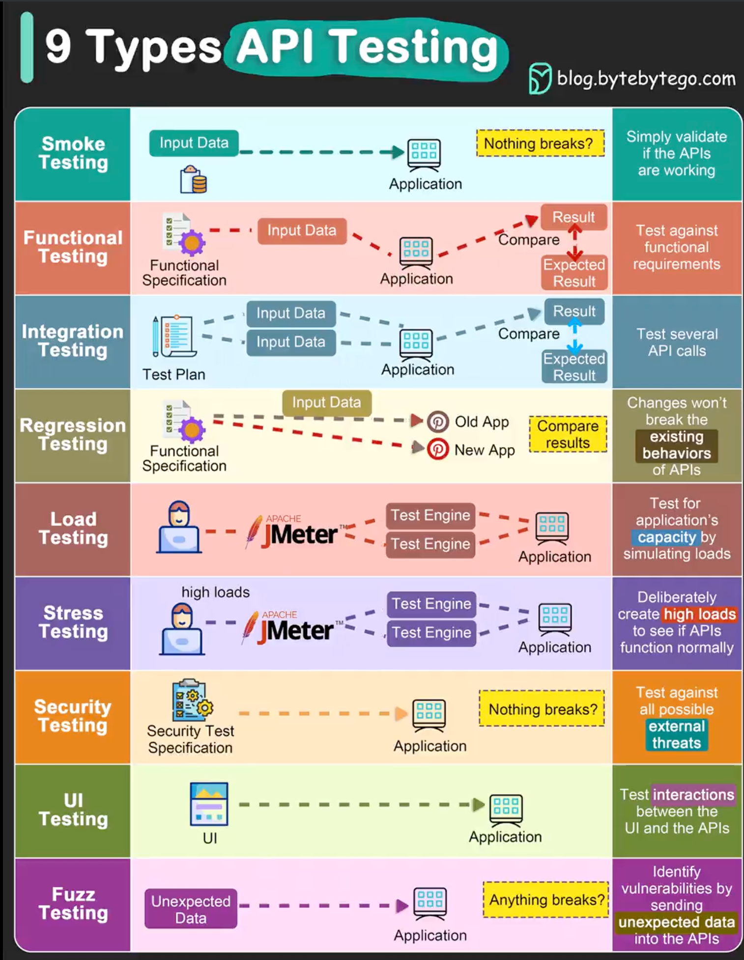
src:blog.bytebytego.com
Smoke Testing is done after API development is complete. It simply validates whether the APIs are working and nothing breaks.
Functional Testing This creates a test plan based on the functional requirements and compares the results with the expected results.
Integration Testing This test combines several API calls to perform end-to-end tests. It also tests intra-service communications and data transmissions.
Regression Testing This test ensures that bug fixes or new features shouldn’t break the existing behaviors of APIs.
Load Testing To understand the system’s behavior under a specific expected load. It’s mainly concerned with normal operational conditions.
Stress Testing To understand the limits of the system and how it behaves under extreme conditions. It’s designed to test the system beyond its standard operational capacity, often to a breaking point, to see how it handles stress or overload.
Security Testing This tests the APIs against all possible external threats.
UI Testing This tests the UI interactions with the APIs to ensure the data can be displayed correctly.
Fuzz Testing This injects invalid or unexpected input data into the API and tries to crash the API. In this way, it identifies the API vulnerabilities.
YT Video
https://www.youtube.com/watch?v=qquIJ1Ivusg
[Avg. reading time: 3 minutes]
Flask Demo Testing
-v : Verbose mode. Shows detailed test results when both Success/Failure.
uv run python -m unittest tests/test_01.py -v

or

poetry run python -m unittest tests/test_01.py -v
uv run python -m unittest tests/test_02.py -v

or

poetry run python -m unittest tests/test_02.py -v
uv run python -m unittest tests/test_03.py -v

or

poetry run python -m unittest tests/test_03.py -v
uv run python  -m unittest tests/test_04.py -v

or

poetry run python  -m unittest tests/test_04.py -v
To run all test files in one go
uv run python  -m unittest discover tests -v

or

poetry run python  -m unittest discover tests -v
To test based on pattern
uv run python  -m unittest tests/t*_04*.py -v

or

poetry run python  -m unittest tests/t*_04*.py -v
To skip a partition function inside a file
@unittest.skip() - to skip a particular test
[Avg. reading time: 6 minutes]
NoSQL Databases
[Avg. reading time: 9 minutes]
Types of NoSQL Databases
| Database Type | Examples |
|---|---|
| Document Store | MongoDB (Open Source) CouchDB (Open Source) |
| Key-Value Store | Redis (Open Source) DynamoDB (Commercial) |
| Wide-Column Store | Cassandra (Open Source) HBase (Open Source) |
| Graph Database | Neo4j (Open Source / Commercial) OrientDB (Open Source) |
| Time Series Database | InfluxDB (Open Source) TimescaleDB (Open Source / Commercial) |
| Multi Model Database | FaunaDB (Commercial) ArangoDB (Open Source) |
Key-Value Store
Description: Stores data as a collection of key-value pairs where a key serves as a unique identifier. Highly efficient for lookups, insertions, and deletions.
Examples:
Redis (Open Source): An in-memory data structure store used as a database, cache, and message broker.
DynamoDB (Commercial) is a fully managed, serverless, key-value NoSQL database designed for internet-scale applications provided by AWS.
Document Store
Description: It stores data in documents (typically JSON, BSON, etc.) and allows nested structures. It is ideal for storing, retrieving, and managing document-oriented information.
Examples:
MongoDB (Commercial) is a document database with the scalability and flexibility you want, as well as the querying and indexing you need.
CouchDB (Open Source) is a database that uses JSON for documents, JavaScript for MapReduce indexes, and regular HTTP for its API.
Wide-Column Store
Description: It stores data in tables, rows, and dynamic columns. It is efficient for querying large datasets and suitable for distributed computing.
Examples:
Cassandra (Open Source) is a distributed database system for handling large amounts of data across many commodity servers.
HBase (Open Source) is an open-source, distributed, versioned, non-relational database modeled after Google's Big Table.
Graph Database
Description: Stores data in nodes and edges, representing entities and their interrelations. Ideal for analyzing interconnected data and complex queries.
Examples:
Neo4j (Open Source / Commercial) is a graph database platform that provides an ACID-compliant transactional backend for your applications.
OrientDB (Open Source) is a multi-model database that supports graph, document, object, and key/value models.
Time Series DB
Description: Optimized for handling time-stamped data. Ideal for analytics over time-series data like financial data, IoT sensor data, etc.
Examples:
InfluxDB (Open Source): An open-source time series database that handles high write and query loads.
TimescaleDB (Open Source / Commercial) is an open-source time-series SQL database optimized for fast ingest and complex queries.
Multi-Model DB
Description: Supports multiple data models against a single, integrated backend. This can include documents, graphs, key values, in-memory, and search engines.
Examples:
Redis (with Extensions)
FaunaDB (Commercial): A distributed database that supports multiple data models and is designed for serverless applications.
ArangoDB (Open Source) is a native multi-model database with flexible data models for documents, graphs, and key values.
#nosql #keyvalue #document #graph #columnar #opensource
[Avg. reading time: 3 minutes]
Redis
Redis (Remote Dictionary Server) is an in-memory data structure store.
Primarily prioritizes Consistency and Partition Tolerance when configured in a distributed setup (like Redis Cluster).
Redis is categorized as a key value store within the NoSQL database types.
Key Features
Speed: Redis stores data in the RAM, making it extremely fast.
Persistence Options: Provides options to save data to disk, ensuring durability even after restarts or crashes.
Scalability: Can scale horizontally with Redis Cluster, distributing data across multiple nodes.
Wide Use Cases: This is ideal for scenarios requiring quick data access, such as caching, session management, real-time analytics, and gaming leaderboards.
Advanced Features: Supports advanced features like transactions, pub/sub messaging systems, Lua scripting, and more.
Atomic Operations: Supports transactions and atomic operations.
Data Structures: Supports many data structures, such as
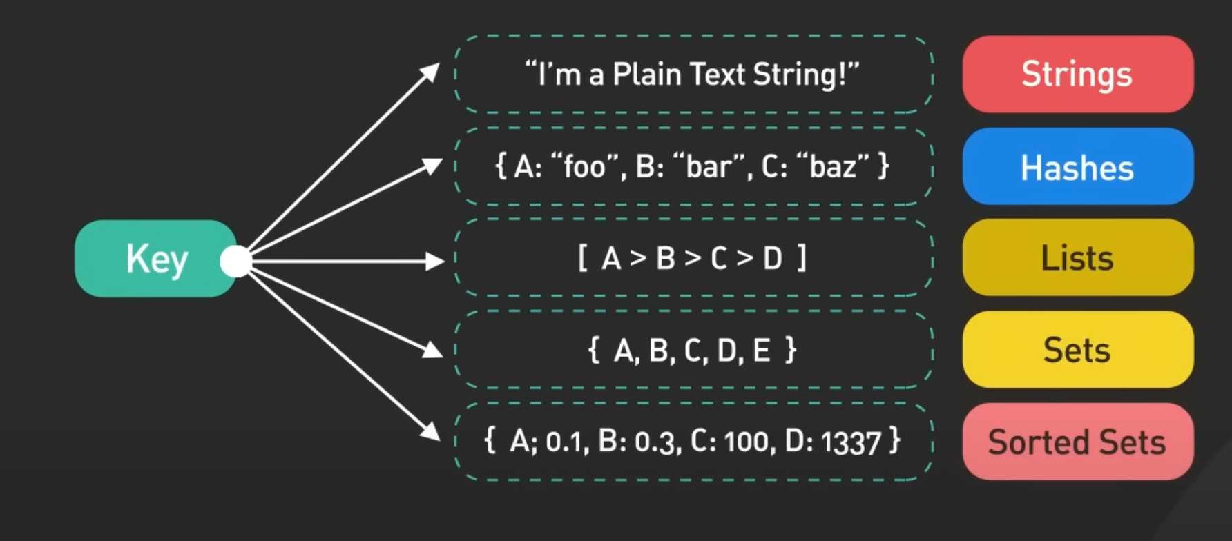
src: bytebytego.com
[Avg. reading time: 11 minutes]
Terms to know
The Redis server is the heart of the Redis system, handling all data storage, processing, and management tasks.
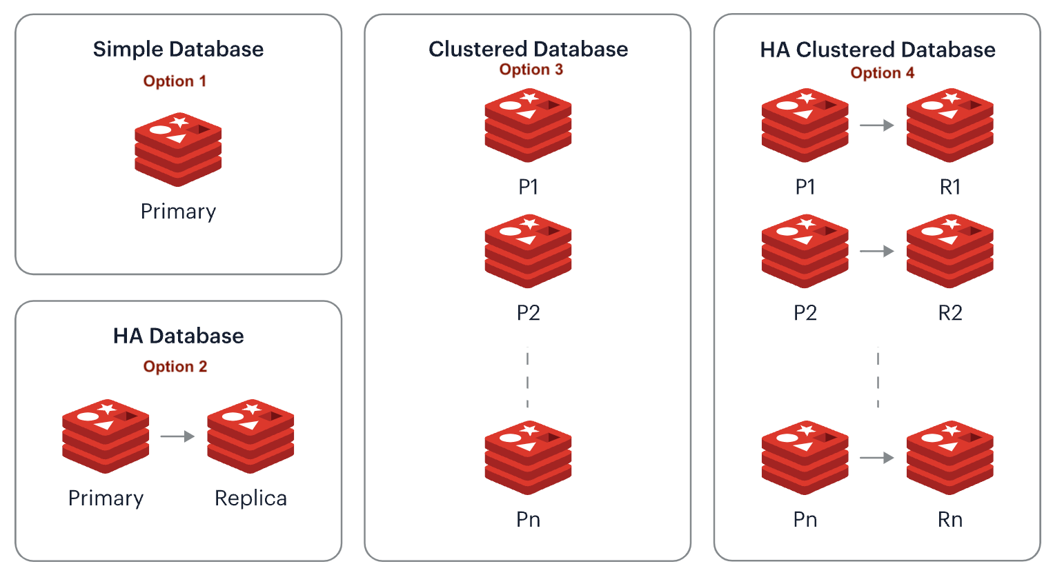
- A simple database, i.e., a single primary shard.
- A highly available (HA) database, i.e., a pair of primary and replica shards.
- A clustered database contains multiple primary shards, each managing a subset of the dataset.
- An HA clustered database, i.e., multiple pairs of primary/replica shards.
Shard: Splitting data across multiple Redis instances to distribute load and data volume. It's like breaking a big dataset into smaller, manageable pieces.

def get_shard(key, total_shards=3):
    # Simple hash function to determine shard
    hash_value = hash(key)
    shard_number = hash_value % total_shards
    print(f"shard:{shard_number}")

get_shard("user:1001")
get_shard("user:1002")
get_shard("user:1003")
get_shard("user:1004")
get_shard("user:1005")
get_shard("user:1006")
get_shard("user:1007")
Cluster: A group of Redis nodes that share data. Provides a way to run Redis where data is automatically sharded across nodes.
Replication is copying data from one Redis server to another for redundancy and scalability. The primary server's data is replicated to one or more secondary (replica) servers.
Transactions: Grouping commands to be executed as a single isolated operation, ensuring atomicity.
Atomicity - The most important reason to use transactions is that they guarantee all commands will be executed together without any other client's commands interrupting them.
Consistency in reads - Within a transaction, you get a consistent view of the data. Commands see the data as it was when the transaction started, not as it changes during the transaction.
Batch operations - Transactions reduce network overhead by sending multiple commands in a single request, which improves performance.
Optimistic locking with WATCH - When combined with the WATCH command, transactions provide a way to ensure data hasn't changed since you last read it.
No Rollbacks
Pipeline: Bundling multiple commands to reduce request/response latency. Commands are queued and executed at once.
Persistence: Saving data to disk for durability. Redis offers RDB (snapshotting) and AOF (logging every write operation).
RDB (Redis Database)
RDB periodically creates point-in-time snapshots of your dataset at specified intervals. It is generally faster for larger datasets because it doesn't write every disk change, reducing I/O overhead.
AOF (Append Only File)
Durability: Records every write operation received by the server. You can configure the fsync policy to balance between durability and performance.
Data Loss Risk: Less risk of data loss compared to RDB. It can be configured to append each operation to the AOF file as it happens or every second.
Recovery Speed: Slower restarts compared to RDB because Redis replays the entire AOF to rebuild the state.
Multi-Model Database
- Redis-Core - Key-Value Store
- Extend with Redis Modules
- Redis Search - Elastic Search
- RedisGraph - Graph Database
- RedisJSON - Document Database
- RedisTimeSeries - TimeSeries Database
#redis #keywords #redisgraph #redisshard
[Avg. reading time: 6 minutes]
Redis - (RDBMS) MySql
Can Redis replace MySQL?
MySQL:
- A relational database management system (RDBMS).
- Uses structured query language (SQL) for database access.
- Ideal for complex queries and joins.
- Data is stored in tables with rows and columns.
- ACID-compliant (Atomicity, Consistency, Isolation, Durability).
Redis:
- An in-memory data structure store.
- Not a traditional RDBMS, but a NoSQL database.
- Data is stored as key-value pairs.
- Fast performance due to in-memory storage.
- There is limited support for complex queries and no support for joins.
Similarities:
- Data Storage: Both can store data, but Redis does so in memory and is more limited in data types.
- Persistence: Redis offers persistence mechanisms, allowing it to store data permanently like MySQL.
Differences:
- Data Modeling: Redis doesn't support relational data modeling. Data relationships are managed differently, often requiring denormalization or secondary indexing.
- Remember 1 - 1, 1 - n, n - n mapping?
- Query Capability: Redis has limited query capabilities compared to MySQL. It doesn't support SQL or complex queries involving multiple tables.
Scenarios where Redis can be used like MySQL:
- Simple Data Storage: For applications that require simple key-value data storage.
- Caching: Redis is often used alongside MySQL to cache query results, reducing load on the MySQL database.
- Session Storage: Storing user session data doesn't require complex querying.
- Queue Systems: Implementing queues for message brokering, which is not a typical use case for MySQL.
So, can Redis finally replace MySQL?

While Redis can handle some database functionalities similar to MySQL, it's not a complete replacement for a relational database system. Redis is often used with databases like MySQL to leverage its fast caching, session storage, and real-time operations performance.
[Avg. reading time: 2 minutes]
Redis Cache Demo
Fork and Clone
git clone https://github.com/gchandra10/python_flask_redis_mysql_demo.git
Rename config.yaml.template file to config.yaml
mysql:
  host: localhost
  user: yourusername
  password: yourpassword
  port: mysqlport

redis:
  host: redis_host_name
  db: 0
  user: default
  password: redis_password
  port: redis_port
Remember, by default, redis starts with db:0 and user: default.
Unless you specifically create a new one.
uv run python app.py

or

poetry run python app.py

or

python app.py
Navigate to
http://127.0.0.1:8000
Now call http://127.0.0.1:8000/film/1
The request will be made from MySQL
Refreshing it again, it will be from Redis.
Check the Time taken to load the data.
[Avg. reading time: 1 minute]
Redis Use Cases
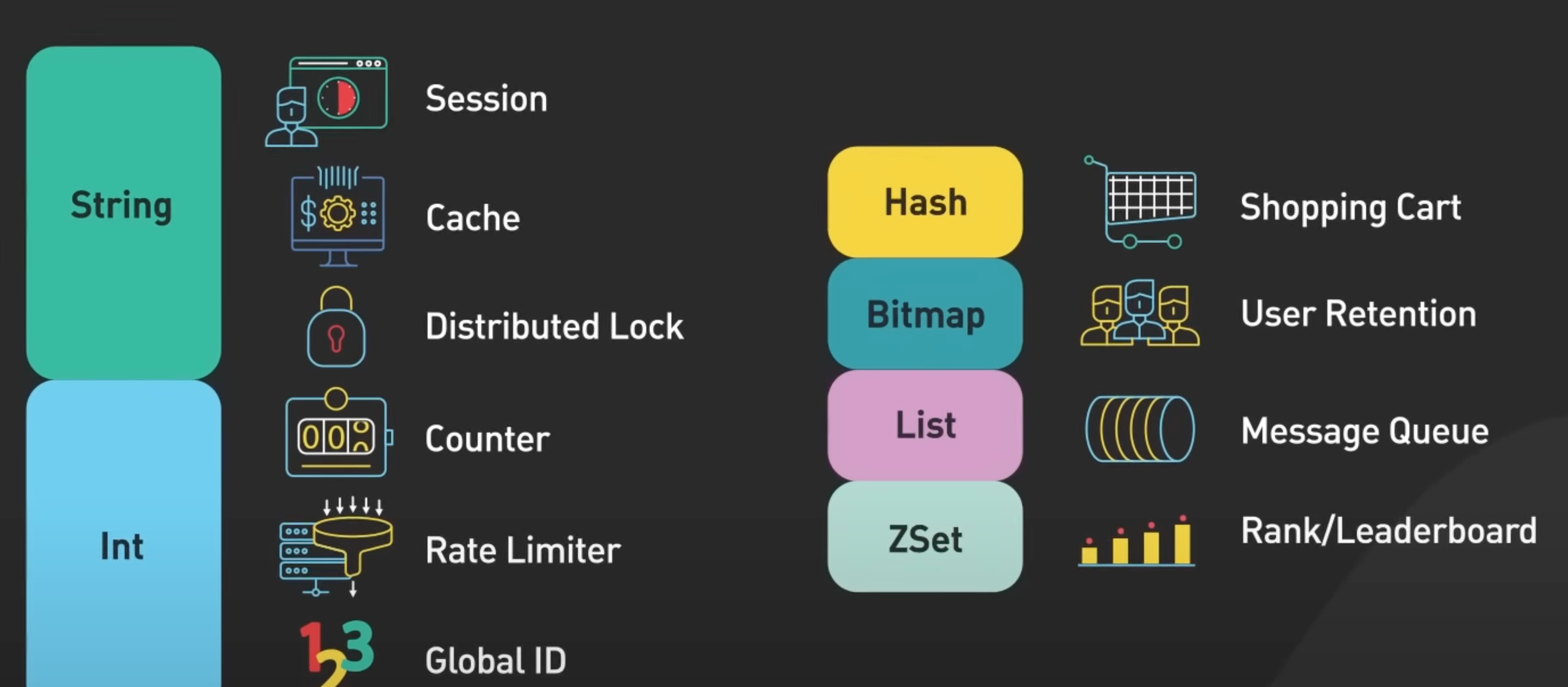
bytebytego.com
Caching:

Rate Limiter: - Used in API
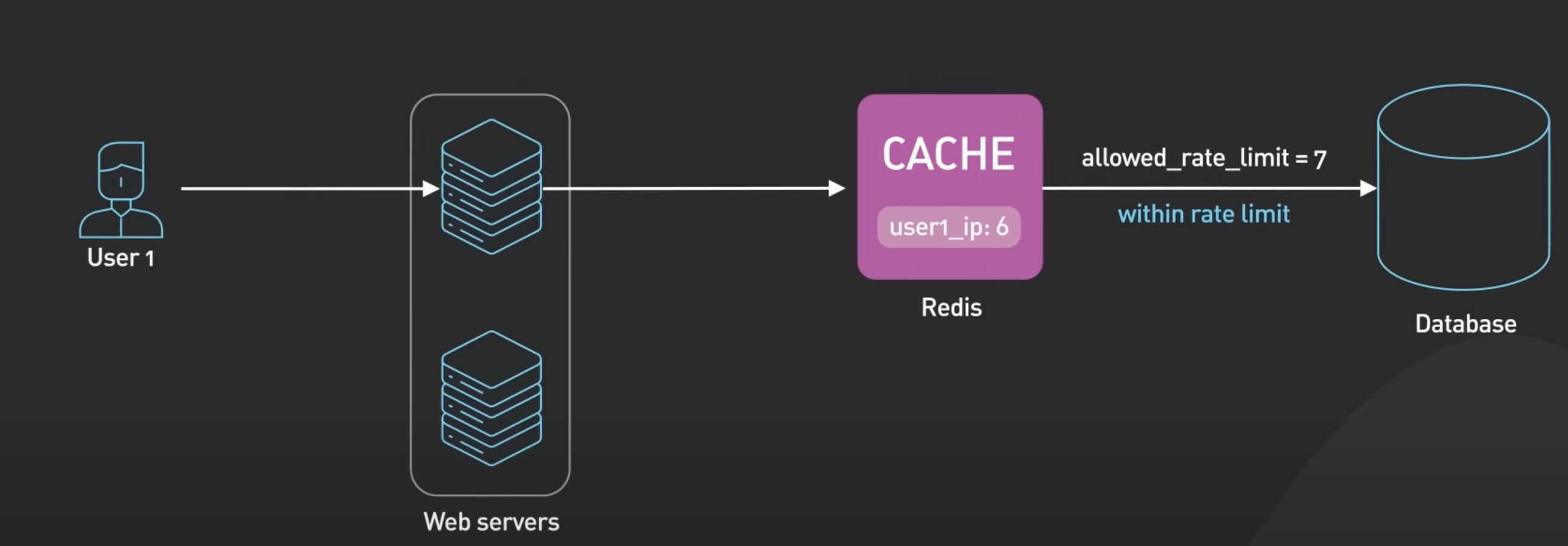
Rank/Leaderboard

[Avg. reading time: 4 minutes]
Databases
In Redis, databases are identified by integer indices, not by unique names as in some other database systems. By default, Redis configures 16 separate databases (numbered from 0 to 15), and you can select a database using the SELECT command followed by the database index.
By default its db 0
Legacy Feature still available for backward compatibility
To switch to another database
SELECT <db number>

SELECT 1
Data Isolation: While Redis supports multiple databases, the separation is relatively thin. All databases share the same Redis instance resources (memory, CPU, etc.), and commands that operate on the server or affect the global state (like FLUSHALL or CONFIG) will affect all databases.
Use in Production: Multiple databases within a single Redis instance are less common in production environments. Instead, it's often recommended to use separate Redis instances for data that needs to be logically separated, as this approach provides stronger data isolation and can prevent one application's data from impacting another.
Persistence and Backup: Be aware that RDB and AOF persistence files contain data from all databases in the Redis instance. If you're using persistence, backing up or restoring these files will back up or restore data for all databases, not just one.
Clear Memory
    flushdb - clears the current database.
    flushall - clears all the databases.
#database #flushdb #flushall #RDB #AOF
[Avg. reading time: 0 minutes]
Data Structures
[Avg. reading time: 8 minutes]
Strings
Single Namespace
SET "rachel" "Fashion"
GET "rachel"
STRLEN "rachel"
APPEND "rachel" " Designer"

GET "rachel"

#get first 5 letters
GETRANGE "rachel" 0 4

#Skip last 2 (extreme right is -1 and -2 and so on)
GETRANGE "rachel" 0 -3

# Substring
GETRANGE "rachel" 5 8

# Get the last 5 letters

GETRANGE "rachel" -5 -1
Two Namespaces
SET "character:rachel" "Fashion"
GET "character:rachel"
STRLEN "character:rachel"

APPEND "character:rachel" " Designer"
GET "character:rachel"
GETRANGE "character:rachel" 0 4

SET "character:ross" "Palentologist"
SET "character:chandler" "Accountant"
SET "character:joey" "Actor"

-- Returns all the characters
Option 1:

SCAN 0 MATCH "character:*" COUNT 10

Option 2:

KEYS character:*
Using SCAN is non blocking, allowes other commands to be processed between iterations. Iterates the key space incrementally.
Using KEYS will block the server when scanning for all the data. Returns all matching keys in a single operation. This might lead to latency in large databases and can affect other users. It is not to be used in Production.
Three Namespaces
SET "character:rachel:job" "Fashion"
SET "character:rachel:lastname" "Green"
SET "character:rachel:gender" "Female"
SET "character:rachel:age" 30

SET "character:ross:job" "Palentologist"
SET "character:ross:lastname" "Geller"
SET "character:ross:gender" "Male"
SET "character:ross:age" 32

SET "character:chandler:job" "Accountant"
SET "character:chandler:lastname" "Bing"
SET "character:chandler:gender" "Male"
SET "character:chandler:age" 32

GET "character:rachel:job"
STRLEN "character:rachel:job"
APPEND "character:rachel:job" " Designer"
GETRANGE "character:rachel:job" 0 4

KEYS "character:*:job"

KEYS "character:ross:*"

DEL "character:chandler"

EXISTS "character:chandler"
-
SETNX: Sets the value of a key only if the key does not exist.
SETNX "character:rachel" "Fashion" -
SETEX: Sets the value of a key with an expiration time.
SETEX "character:rachel" 60 "Fashion"(expires in 60 seconds) -
MSET: Sets multiple keys to multiple values in a single atomic operation.
MSET "character:rachel" "Fashion" "character:ross" "Paleontologist" -
MGET: Gets the values of all the given keys.
MGET "character:rachel" "character:ross" -
INCR: Increments the integer value of a key by one.
INCR "pageviews:rachelProfile"GET "pageviews:rachelProfile" -
DECR: Decrements the integer value of a key by one.
DECR "stock:centralPerkMugs" -
INCRBY: Increments the integer value of a key by the given amount.
INCRBY "followers:rachel" 10 -
DECRBY: Decrements the integer value of a key by the given number.
DECRBY "debt:rachel" 100 -
INCRBYFLOAT: Increments the float value of a key by the given amount.
INCRBYFLOAT "balance:rachel" 100.50 -
GETSET: Sets a new value and returns the old value.
GETSET "character:rachel" "Executive" -
MSETNX: Sets multiple keys to multiple values only if none exist.
MSETNX "character:rachel" "Fashion" "character:monica" "Chef" -
PSETEX: Similar to
SETEXPSETEX but with an expiration time in milliseconds.PSETEX "character:rachel" 60000 "Fashion"(expires in 60,000 milliseconds or 60 seconds)
#Strings #Namespaces #NoSQL #Redis
[Avg. reading time: 9 minutes]
List
Redis lists are linked lists of string values. Redis lists are frequently used to:
- Implement stacks and queues.
- Build queue management for background worker systems.
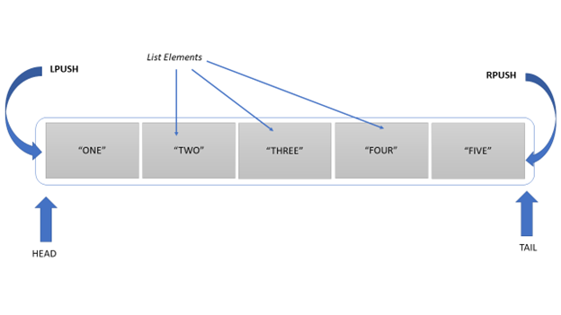
src: https://linuxhint.com/redis-lpop/
-
LPUSHadds a new element to the head of a list;RPUSHadds to the tail. -
LPOPremoves and returns an element from the head of a list;RPOPdoes the same but from the tails of a list. -
LLENReturns the length of a list. -
LMOVEAtomically moves elements from one list to another. -
LTRIMReduces a list to the specified range of elements.
FIFO: First In, First Out
LIFO: Last In, First Out
Adding Tasks to the Queue
Use the LPUSH or RPUSH command to add new tasks to the list. Here, we'll use RPUSH to ensure tasks are added to the end of the list.
RPUSH task_queue "Task 1: Process image A"
RPUSH task_queue "Task 2: Send email to user B"
RPUSH task_queue "Task 3: Generate report for user C"
Sort Alphabets with ALPHA
SORT task_queue ALPHA
Processing Tasks from the Queue
Use the LPOP command to remove and get the first element from the list. This simulates processing the tasks in the order they were received.
Pops the first value: "Task 1: Process image A"
LPOP task_queue
Length of the Queue
LLEN task_queue
Use the LRANGE command to view tasks
LRANGE task_queue 0 -1
More Use Cases
Chat Application: Use lists to store messages in a chat room. Each message can be pushed to the list, and the latest messages can be displayed using LRANGE.
Activity Logs: Maintain an activity log where each action is pushed to the list. You can then retrieve the latest actions by using LRANGE or delete old ones using LTRIM.
Real-Time Leaderboard: Keep a list of top scores in a game. Push scores to the list and trim it to keep only the top N scores using LTRIM.
Try these examples
LPUSH user:123:activity "Viewed product 456"
LPUSH user:123:activity "Added product 789 to cart"
LPUSH user:123:activity "Checked out order 321"
Limit Activity Log to Last N Items Truncates the list to last 10 items. Others are deleted.
LTRIM user:123:activity 0 9
Get Recent Activities This is readonly.
LRANGE user:123:activity 0 -1
Sort
RPUSH mylist 5 3 8 1 6
SORT mylist
#RPUSH #LPUSH #List #NoSQL #Redis
[Avg. reading time: 7 minutes]
Set
A Redis set is an unordered collection of unique strings (members). You can use Redis sets to efficiently:
Key Characteristics of Redis Sets
Uniqueness: Each element in a set is unique. Attempting to add duplicate elements has no effect.
Unordered: Sets do not maintain the order of elements, making them ideal for operations where order does not matter.
-
Track unique items (e.g., track all unique IP addresses accessing a given blog post).
-
Represent relations (e.g., the set of all users with a given role).
-
Perform common set operations such as intersection, unions, and differences.
-
SADDadds a new member to a set. -
SREMremoves the specified member from the set. -
SISMEMBERtests a string for set membership. -
SINTERreturns the set of members that two or more sets have in common (i.e., the intersection). -
SCARDreturns the size (a.k.a. cardinality) of a set.
Tags
SADD post:101:tags "Redis" "Databases" "NoSQL"
SADD post:102:tags "Programming" "Python" "NoSQL"

-- Output the values

SMEMBERS post:101:tags

-- Insection

SINTER post:101:tags post:102:tags

-- Union

SUNION post:101:tags post:102:tags

-- Move

SMOVE post:102:tags post:101:tags "Python"

-- Remove tag

SREM post:101:tags "NoSQL"
User Active Sessions
-- add users

SADD active_users "user:123"
SADD active_users "user:456"
SADD active_users "user:789"

-- checking whether is member

SISMEMBER active_users "user:456"

-- remove user

SREM active_users "user:456"

-- returns total number of items

SCARD active_users
Social Media Example
SADD "user:userID1:followers" followerID1
SADD "user:userID1:followers" followerID2

SADD "user:userID2:followers" followerID1
SADD "user:userID2:followers" followerID3

-- Find the common followers between two users
SINTER "user:userID1:followers" "user:userID2:followers"

-- Get the SET values
SMEMBERS "user:userID1:followers"

-- Gets the size of the set.
SCARD "user:userID1:followers"

-- Find out whether followerID1 is part of this set
SISMEMBER user:userID1:followers followerID1
Use Cases
Real-time Analytics: Track and display unique events or items, like products viewed in a session.
ACLs (Access Control List): Manage user access to certain features or commands.
#SADD #SMEMBERS #ACL #NoSQL #Redis
[Avg. reading time: 6 minutes]
Hash
Redis hashes are record types structured as collections of field-value pairs. You can use hashes to represent basic objects and to store groupings of counters, among other things.
Key Characteristics of Redis Hashes:
Field-Value Storage: Each hash can store multiple fields and values, similar to columns in a relational database.
Efficient Operations: You can read or write specific fields within a hash without retrieving or updating the entire hash.
Compact Storage: Hashes are memory-efficient, especially for storing objects with many fields.
-
HSETsets the value of one or more fields on a hash. -
HGETreturns the value at a given field. -
HMGETreturns the values at one or more given fields. -
HINCRBYincrements the value at a given field by the integer provided.
HSET "product:501" title "Laptop" price "799" description "Latest model..." stock "150"

(Retrieve title and price for the product)
HMGET "product:501" title price stock

(Decrement stock by 1 when a product is purchased)
HINCRBY "product:501" stock -1

HMGET "product:501" title price stock

HGETALL "product:501"

HEXISTS "product:501" title

HDEL "product:501" "stock"
Use Case: User Session Store
| userid | 1 |
|---|---|
| name | Rachel |
| ip | 10.20.133.233 |
| hits | 1 |
HSET usersession:1 userid 1 name Rachel ip 10.20.133.233 hits 1

# One Value
HGET usersession:1 hits

# Multiple Values
HMGET usersession:1 userid name ip hits

# Increment
HINCRBY usersession:1 hits 1

HDEL usersession:1 hits

# What happens when you GET the deleted key?

HMGET usersession:1 userid name ip hits
EXPIRE
Sets a Key's time to live (TTL). The key will be automatically deleted from Redis once a specific duration (in seconds) has elapsed.
EXPIRE usersession:1 10
DEL
Immediately deletes a key and its associated value from Redis
DEL usersession:1
[Avg. reading time: 6 minutes]
Pub/Sub
Redis Pub/Sub (Publish/Subscribe) is a messaging paradigm within Redis that allows for message broadcasting through channels. This feature enables the development of real-time messaging applications by allowing publishers to send messages to an unspecified number of subscribers asynchronously.
Notifications and Alerts
For applications that need to notify users of events in real time (such as social media notifications, stock alerts, or emergency alerts), Redis Pub/Sub provides a lightweight and fast way to distribute messages.
Live Data Updates
In dashboard applications or live data feeds (such as sports scores, financial market data, or IoT sensor data), Redis Pub/Sub can push updates to clients as soon as new data is available.
Decoupling Microservices
Redis Pub/Sub can be a messaging backbone to decouple microservices architectures. Services can publish events or messages without knowing the details of which services are subscribed to those events. This promotes loose coupling, making the system more scalable and easier to maintain.
Limitations
-
- Message Persistence
-
- Lack of Delivery Acknowledgment
-
- Filtering and Routing - Lacks advanced filtering other than basic
-
- Resource Utilization
Because Redis operates in memory, high volumes of messages or large numbers of subscribers can lead to significant memory and network bandwidth usage. Planning and monitoring resource utilization becomes critical as the messaging system grows in scale.
Client 1
subscribe class_update_channel
subscribe school_update_channel
Client 2
psubscribe *_channel bigdata_class_mates
Producer
publish class_update_channel "Hello class"
publish school_update_channel "who is graduating this summer?"
publish glassboro_channel "welcome to Glassboro"
[Avg. reading time: 10 minutes]
Geospatial Index
Proximity Searches: These find items close to a given point, such as the nearest restaurants to a user's location.
Radius Queries: These queries retrieve items within a specific distance from a point. They are useful for services like delivery area checks or local event discovery.
Distance Calculation: Calculate the distance between two geo points.
GEOADD to add a point GEODIST to find the distance between two points GEOSEARCH to find all points within a radius
GEOADD locations -75.1118 39.7029 Glassboro
GEOADD locations -75.2241 39.7393 MullicaHill
GEOADD locations -75.3105 39.7476 Swedesboro
GEOADD locations -75.2404259 39.8302 Paulsboro
GEOADD locations -75.0246 39.9268 CherryHill
GEOADD locations -74.9489 39.9689 Moorestown

## Straight Line or As-The-Crow-flies

GEODIST locations Glassboro MullicaHill mi
GEODIST locations CherryHill Moorestown mi
GEODIST locations CherryHill Moorestown km

## Find nearby areas

GEORADIUS locations -75.1118 39.7029 15 mi

GEOADD locations:restaurant -75.11486 39.72257 'Italian Affiar Restaurant'
GEOADD locations:restaurant -75.11275 39.70404 'LaScala Fire Glassboro'
GEOADD locations:restaurant -75.11333 39.70519 'Mexican Mariachi Grill'
GEOADD locations:pharmacy -75.13068 39.73228 'Pitman Pharmacy'
GEOADD locations:pharmacy -75.09853 39.68319 'Walgreens Pharmacy'

## Get nearby Restaurant & Pharmacy

GEORADIUS locations:restaurant -75.1118 39.7029 5 mi
GEORADIUS locations:pharmacy -75.1118 39.7029 2 mi
GEOSEARCH is same as GEORADIUS but cleaner syntax.
GEOSEARCH locations:cities FROMMEMBER Glassboro BYRADIUS 10 mi

GEOPOS locations:cities Moorestown
https://www.mapsofworld.com/usa/states/new-jersey/lat-long.html
Using GEOADD command to add geospatial data (latitude, longitude, and a member), Redis internally converts the latitude and longitude into a geohash. This geohash is then stored as the score in a sorted set, with the member name as the value. The sorted set allows for efficient querying of geospatial data, such as finding nearby locations.
GeoHash
Geohashing is a method of encoding geographic coordinates (latitude and longitude) into a compact string of letters and digits. This string represents a specific rectangular area on Earth, with higher precision obtained by increasing the length of the geohash. It essentially divides the world into a grid, with each geohash representing one of the grid cells.
Demonstrate how world is split into Grid :)
OR
Search this place: dr49fg9q0hyx
GEOHASH locations CherryHill
Advantages
Proximity Search Optimization: Geohashes group nearby locations together by design. Locations with similar geohash prefixes are spatially close, allowing proximity searches to be performed more efficiently by simply comparing prefixes instead of calculating distances for every entry.
Efficient Indexing: Geohashes are simple alphanumeric strings that can be indexed using common database structures (like sorted sets or hash maps). This makes geohashes easier to index and search, reducing the complexity of querying nearby points.
Grid System for Clustering: The geohash grid system clusters nearby points by their geohash values. If you want to visualize or process areas in terms of spatial grids, geohashing provides a clean and efficient method of doing so.
Compact Representation: A geohash is a single compact alphanumeric string that represents both latitude and longitude in a single value. This saves space in databases and simplifies the process of querying and storing location data.
[Avg. reading time: 1 minute]
Redis - Python
Fork and Clone
git clone https://github.com/gchandra10/python_redis_examples.git
Install Poetry
cd python_redis_examples
uv sync

or

poetry update
uv run python 01_string.py
uv run python 02_string.py
uv run python 03_list.py
...
...
OR
poetry run python 01_string.py
poetry run python 02_string.py
poetry run python 03_list.py
...
...
#python #redis_python #examples
[Avg. reading time: 7 minutes]
Redis JSON
Redis Stack extends the core features of Redis OSS and provides a complete developer experience for debugging and more.
- RedisJSON
- RedisGraph
- RedisTimeseries
- RedisSearch
The JSON capability of Redis Stack provides JavaScript Object Notation (JSON) support for Redis. It lets you store, update, and retrieve JSON values in a Redis database, similar to any other Redis data type.
JSON.SET friends:character:rachel $ '{"name": "Rachel Green", "occupation": "Fashion Executive", "relationship_status": "Single", "friends": ["Ross Geller", "Monica Geller", "Joey Tribbiani", "Chandler Bing", "Phoebe Buffay"] }'
Dollar sign ($) represents the Root node
JSON.GET friends:character:rachel
Retrieve Specific fields
JSON.GET friends:character:rachel $.name $.occupation
Adds education at the end
JSON.SET friends:character:rachel $.education '
{"high_school": "Lincoln High School", "college": "Not specified" }'
JSON.GET friends:character:rachel
Adding Array of values
JSON.SET friends:character:rachel $.employment_history '[ { "company": "Central Perk", "position": "Waitress", "years": "1994-1995" }, { "company": "Bloomingdale\'s", "position": "Assistant Buyer", "years": "1996-1999" }, { "company": "Ralph Lauren", "position": "Executive", "years": "1999-2004" } ]'
Get Employment History
json.get friends:character:rachel employment_history
JSON.GET friends:character:rachel $.employment_history[*].company
Get specific one
json.get friends:character:rachel employment_history[1]
Scan All Keys
SCAN 0 MATCH friends:character:*
Add more data
JSON.SET friends:character:ross $ '{
  "name": "Ross Geller",
  "occupation": "Paleontologist",
  "relationship_status": "Divorced",
  "friends": ["Rachel Green", "Monica Geller", "Joey Tribbiani", "Chandler Bing", "Phoebe Buffay"],
  "children": [
    {
      "name": "Ben Geller",
      "mother": "Carol Willick"
    },
    {
      "name": "Emma Geller-Green",
      "mother": "Rachel Green"
    }
  ],
  "education": {
    "college": "Columbia University",
    "degree": "Ph.D. in Paleontology"
  }}'
JSON.SET friends:character:monica $ '{
  "name": "Monica Geller",
  "occupation": "Chef",
  "relationship_status": "Married",
  "friends": ["Ross Geller", "Rachel Green", "Joey Tribbiani", "Chandler Bing", "Phoebe Buffay"],
  "spouse": "Chandler Bing",
  "education": {
    "culinary_school": "Not specified"
  },
  "employment_history": [
    {
      "company": "Alessandro\'s",
      "position": "Head Chef",
      "years": "Not specified"
    },
    {
      "company": "Javu",
      "position": "Chef",
      "years": "Not specified"
    }
  ]}'
JSON.GET friends:character:ross $.name $.occupation
JSON.SET friends:character:chandler $ '{
  "name": "Chandler Bing",
  "occupation": "Statistical analysis and data reconfiguration",
  "relationship_status": "Married",
  "friends": ["Ross Geller", "Monica Geller", "Joey Tribbiani", "Rachel Green", "Phoebe Buffay"],
  "spouse": "Monica Geller",
  "education": {
    "college": "Not specified"
  }}'
JSON.SET friends:character:phoebe $ '{
  "name": "Phoebe Buffay",
  "occupation": "Masseuse and Musician",
  "relationship_status": "Married",
  "friends": ["Ross Geller", "Monica Geller", "Joey Tribbiani", "Chandler Bing", "Rachel Green"],
  "spouse": "Mike Hannigan",
  "education": {
    "high_school": "Not completed"
  }}'
JSON.SET friends:character:joey $ '{
  "name": "Joey Tribbiani",
  "occupation": "Actor",
  "relationship_status": "Single",
  "friends": ["Ross Geller", "Monica Geller", "Chandler Bing", "Rachel Green", "Phoebe Buffay"],
  "education": {
    "drama_school": "Not specified"
  },
  "employment_history": [
    {
      "show": "Days of Our Lives",
      "role": "Dr. Drake Ramoray",
      "years": "Various"
    }
  ]}'
Delete specific node
JSON.DEL friends:character:monica $.occupation
[Avg. reading time: 20 minutes]
Redis Search
Redis Search (or RediSearch) is a full-text search and secondary indexing engine for Redis. It allows for performing complex searches and filtering over the data stored in Redis without needing a relational database. This powerful module enables advanced querying capabilities like full-text search, filtering, aggregation, and auto-complete.
Key Features
Full-text Search: Perform text searches with support for stemming, phonetic matching, and ranked retrieval.
Secondary Indexing: Create indexes for quick lookup of data stored in Redis.
Complex Querying: Supports boolean logic, fuzzy matching, numeric filtering, and geospatial querying.
Autocomplete: Typeahead and autocomplete functionalities for building responsive applications.
Faceted Search and Aggregation: Aggregate results and perform statistical queries like grouping and sorting.
Use Cases
E-commerce Platforms:
Search through product descriptions, tags, and categories.
Use filters like price, category, or brand with full-text search for a better user experience.
Content Management Systems:
Implement full-text search for articles, blogs, and documents.
Provide auto-complete for faster and more user-friendly search results. Log and Event Analysis:
Search and filter through logs stored in Redis.
Perform real-time querying and analytics for log monitoring systems.
Geospatial Applications:
Combine geospatial search (e.g., find nearby stores) with text search capabilities. Ideal for applications like food delivery or finding services near a user location.
Chat and Messaging Applications:
Index and search chat messages.
Allow searching through conversations with fuzzy matching and keyword highlights.
User Profiles and Recommendations:
Search user attributes or interests to provide personalized content or recommendations.
Quickly index and lookup attributes like hobbies, location, and preferences.
flushdb
JSON.SET friends:character:ross $ '{
  "name": "Ross Geller",
  "occupation": "Paleontologist",
  "relationship_status": "Divorced",
  "friends": ["Rachel Green", "Monica Geller", "Joey Tribbiani", "Chandler Bing", "Phoebe Buffay"],
  "children": [
    {
      "name": "Ben Geller",
      "mother": "Carol Willick"
    },
    {
      "name": "Emma Geller-Green",
      "mother": "Rachel Green"
    }
  ],
  "education": {
    "college": "Columbia University",
    "degree": "Ph.D. in Paleontology"
  }}'

JSON.SET friends:character:monica $ '{
  "name": "Monica Geller",
  "occupation": "Chef",
  "relationship_status": "Married",
  "friends": ["Ross Geller", "Rachel Green", "Joey Tribbiani", "Chandler Bing", "Phoebe Buffay"],
  "spouse": "Chandler Bing",
  "education": {
    "culinary_school": "Not specified"
  },
  "employment_history": [
    {
      "company": "Alessandro\'s",
      "position": "Head Chef",
      "years": "Not specified"
    },
    {
      "company": "Javu",
      "position": "Chef",
      "years": "Not specified"
    }
  ]}'

JSON.SET friends:character:chandler $ '{
  "name": "Chandler Bing",
  "occupation": "Statistical analysis and data reconfiguration",
  "relationship_status": "Married",
  "friends": ["Ross Geller", "Monica Geller", "Joey Tribbiani", "Rachel Green", "Phoebe Buffay"],
  "spouse": "Monica Geller",
  "education": {
    "college": "Not specified"
  }}'

JSON.SET friends:character:phoebe $ '{
  "name": "Phoebe Buffay",
  "occupation": "Masseuse and Musician",
  "relationship_status": "Married",
  "friends": ["Ross Geller", "Monica Geller", "Joey Tribbiani", "Chandler Bing", "Rachel Green"],
  "spouse": "Mike Hannigan",
  "education": {
    "high_school": "Not completed"
  }}'

JSON.SET friends:character:joey $ '{
  "name": "Joey Tribbiani",
  "occupation": "Actor",
  "relationship_status": "Single",
  "friends": ["Ross Geller", "Monica Geller", "Chandler Bing", "Rachel Green", "Phoebe Buffay"],
  "education": {
    "drama_school": "Not specified"
  },
  "employment_history": [
    {
      "show": "Days of Our Lives",
      "role": "Dr. Drake Ramoray",
      "years": "Various"
    }
  ]}'

JSON.SET friends:guest:janice $ '{
  "name": "Janice Litman Goralnik",
  "occupation": "Unknown",
  "relationship_status": "Divorced",
  "catchphrase": "Oh. My. God!",
  "friends": ["Chandler Bing"],
  "appearances": [
    {
      "season": 1,
      "episode": 5
    },
    {
      "season": 2,
      "episode": 3
    },
    {
      "season": 3,
      "episode": 8
    },
    {
      "season": 4,
      "episode": 13
    },
    {
      "season": 5,
      "episode": 11
    },
    {
      "season": 7,
      "episode": 7
    },
    {
      "season": 10,
      "episode": 15
    }
  ]}'

JSON.SET friends:guest:gunther $ '{
  "name": "Gunther",
  "occupation": "Chef",
  "relationship_status": "Single",
  "workplace": "Central Perk",
  "crush": "Rachel Green",
  "friends": ["Rachel Green", "Joey Tribbiani", "Monica Geller", "Ross Geller", "Phoebe Buffay", "Chandler Bing"],
  "appearances": [
    {
      "season": 1,
      "episode": 2
    },
    {
      "season": 2,
      "episode": 18
    },
    {
      "season": 3,
      "episode": 7
    },
    {
      "season": 5,
      "episode": 2
    },
    {
      "season": 6,
      "episode": 9
    },
    {
      "season": 7,
      "episode": 4
    }
  ]}'
For searching first you have to create INDEXES
FT.CREATE {index_name} ON JSON SCHEMA {json_path} AS {attribute} {type}
<indexName>: The name of the index you are creating.[ON <structure>]: Specifies the data structure to index, which can beHASH(default) orJSONif you're indexing JSON documents with RedisJSON.[PREFIX count <prefix> ...]: Defines one or more key prefixes. Only keys that match the prefix(es) will be indexed.SCHEMA: Followed by one or more field definitions.<field>: The name of the field to index.<type>: The type of the field (TEXT,NUMERIC,GEO, orTAG).
FT.CREATE idx:friends ON JSON PREFIX 1 friends:character: SCHEMA $.name AS name TEXT $.occupation AS occupation TEXT $.relationship_status AS relationship_status TAG
Explanation
idx:friends: Create an index named idx:friends.

ON JSON: Apply this index to JSON documents.

PREFIX 1 friends:character:: Only index keys with this prefix.

SCHEMA: Defines the structure of the index.
$.name AS name TEXT: Index the "name" attribute for full-text search.
$.occupation AS occupation TEXT: Index the "occupation" attribute for full-text search.
$.relationship_status AS relationship_status TAG: Index the "relationship_status" attribute for efficient categorical filtering.
FT.SEARCH idx:friends "@occupation:Chef"
This will return
- Total Number of search results.
- Key of the document.
- Key value pairs representing the JSON content.
- $ means entire document
- contains the all the details
Can I have PREFIX 2?
FT.CREATE idx:friends_guests ON JSON PREFIX 2 friends:character: friends:guest: SCHEMA $.name AS name TEXT $.occupation AS occupation TEXT $.relationship_status AS relationship_status TAG
Now running the query against friends_guests, you will notice 2 docs.
FT.SEARCH idx:friends_guests "@occupation:Chef"
To find all characters who are Married
FT.SEARCH idx:friends "@relationship_status:{Married}"
What happens when you search on columns not indexed?
FT.SEARCH idx:friends "@college:Columbia University"
Recreate the Index
FT.DROPINDEX idx:friends

FT.CREATE idx:friends ON JSON PREFIX 1 friends:character: SCHEMA $.name AS name TEXT $.occupation AS occupation TEXT $.relationship_status AS relationship_status TAG $.education.college AS college TEXT
FT.CREATE idx:occupation ON JSON PREFIX 1 "friends:character:" SCHEMA $.occupation AS occupation TEXT
FT.SEARCH idx:occupation "*"

FT.SEARCH idx:occupation "Chef"
FT.INFO idx:occupation
Auto Suggestion with Fuzzy Logic
SUGADD : Autocomplete suggestion dictionary in Redis Search.
last column is the score. Higher scores mean high priority in suggestion.
FT.SUGADD idx:friends_names "Ross Geller" 2
FT.SUGADD idx:friends_names "Rachel Green" 2
FT.SUGADD idx:friends_names "Monica Geller" 2
FT.SUGADD idx:friends_names "Chandler Bing" 2
FT.SUGADD idx:friends_names "Phoebe Buffay" 2
FT.SUGADD idx:friends_names "Joey Tribbiani" 2
FT.SUGADD idx:friends_names "Gunther" 1
FT.SUGADD idx:friends_names "Janice" 1
FT.SUGGET idx:friends_names "Ro" FUZZY WITHSCORES
Now using Fuzzy logic, it determines Ross Geller sounds more closer than other names. Fuzzy option allows slight misspellings, typos giving more flexibility.
1) "Ross Geller"
2) "0.6324555277824402"
3) "Rachel Green"
4) "0.08161024749279022"
5) "Monica Geller"
6) "0.07813586294651031"
7) "Joey Tribbiani"
8) "0.07507050782442093"
Now lets try without Fuzzy
FT.SUGGET idx:friends_names "Ro"
[Avg. reading time: 7 minutes]
Persistence
RDB (Redis Database)
This method takes snapshots of your database at specified intervals. It's efficient for saving a compact, point-in-time snapshot of your dataset. The RDB file is a binary file that Redis can use to restore its state.
SAVE
Synchronous save of the dataset to disk. When Redis starts the save operation, it blocks all the clients until the save operation is complete. NOT RECOMMENDED IN PROD.
BGSAVE
Background SAVE or Asynchronous SAVE. This forks a new process, and the child process writes the snapshot to the disk. It is used in Prod as Redis continues to process commands while the snapshot is being created.
Automation
redis.conf
save 900 1
Saves the datasets every 900 seconds if at least one write operation has occurred.
save 300 10
Saves the datasets every 300 seconds if at least 10 write operations have occurred.
You can have multiple SAVE in redis.conf file for different conditions.
It creates a dump.rdb file (it is configurable to different name in redis.conf)
dbfilename mybackup.rdb
How to load from RDB?
When Redis is restarted, it checks for the RDB file and loads the contents to memory.
AOF (Append Only File)
This method logs every write operation the server receives, appending each operation to a file. This allows for more granular persistence and more durability than RDB, as you can configure Redis to append data on every write operation at the cost of performance. The AOF file can be replayed to reconstruct the state of the data.
# Enable AOF persistence
appendonly yes

# Specify the filename for the AOF file
appendfilename "appendonly.aof"

# Set the fsync policy to balance durability and performance
# 'always' - fsync on every write; most durable but slower
# 'everysec' - fsync every second; good balance (recommended)
# 'no' - rely on OS to decide; fastest but least durable
appendfsync everysec

auto-aof-rewrite-percentage 100 # Rewrite when AOF size
# Automatic rewriting of the AOF file when it grows too big
auto-aof-rewrite-min-size 64mb  # Minimum size for the AOF file to be rewritten
#AOF #Persistence #NoSQL #Redis #RDB
[Avg. reading time: 5 minutes]
Timeseries
RedisTimeSeries is a Redis module that enhances Redis with capabilities to efficiently store and analyze time series data. It's designed to handle time-based data for use cases such as monitoring, IoT, financial data analysis, etc. Below are some key features of RedisTimeSeries:
Key Features
Efficient Data Storage: Optimized for appending time series data with a low storage footprint.
Automatic Compaction: Supports configurable compaction policies (downsampling) to save space.
Time-Series Aggregation: Built-in functions for aggregation (like AVG, SUM, MIN, MAX).
Label-Based Queries: Similar to tags, labels allow you to query sets of time series using metadata.
Retention Policies: You can set a retention period for data to manage memory usage automatically.
High Throughput: Handles millions of inserts per second, making it a good fit for high-frequency data.
Data Compression: Efficiently compresses time series data for reduced memory usage.
What is Epoch Time?
TS.CREATE temperature:room1 RETENTION 60000 LABELS location room1 unit celsius
- 60000 milli seconds
type temperature:room1
DEL temperature:room1
ADD Data to Time Series
TS.ADD temperature:room1 * 22.5
-
- meaning use the system time.
Add few more
TS.ADD temperature:room1 * 21.5

TS.ADD temperature:room1 * 21.45

TS.ADD temperature:room1 * 22.52
Get the values between EPOCH TS
TS.RANGE temperature:room1 1728503705075 1728503757000
- No you cannot use Human Date time
Aggregation
TS.RANGE temperature:room1 0 + INF AGGREGATION avg 60000
By default Upsert not supported
TS.MADD temperature:room1 1728503756138 23.5 temperature:room1 1728503756139 24.0 temperature:room1 1728503756133 21.8
Get values between earliest TS to latest TS for given range
TS.RANGE temperature:room1 - + FILTER_BY_VALUE 21.5 23.5
GET earliest TS only
TS.RANGE temperature:room1 - + COUNT 1
#TSDB #TimeSeries #NoSQL #Redis
[Avg. reading time: 5 minutes]
Neo4J
Neo4j is a graph database that stores data as nodes (entities) and relationships (edges), focusing on the connections between data points. It excels at analyzing complex, highly connected data, such as social graphs, recommendation systems, and fraud networks.
In the context of the CAP theorem, Neo4j prioritizes Consistency (C) and Partition Tolerance (P) over Availability (A). This means Neo4j ensures data correctness across nodes even in distributed setups, sometimes at the cost of short-term availability.
Neo4J Deployments
| Deployment | Description | Use Case |
|---|---|---|
| Standalone | Installed on a single server; simplest setup. | Development, testing, small workloads. |
| Clustering | Multiple nodes for high availability and load balancing. | Production-grade systems requiring uptime. |
| HA/DR | Adds replication for fault tolerance and disaster recovery. | Mission-critical systems. |
| Neo4j Aura (Cloud) | Fully managed Neo4j service by Neo4j Inc. | Quick start, scalable cloud deployments. |
Use Cases
Social Media
Neo4j models complex social interactions such as friends, followers, and likes.
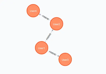
Fraud Detection in Real-time: Banks and financial institutions are leveraging Neo4j to detect complex fraud patterns in real time, connecting the dots between transactions that would seem unrelated at first glance.
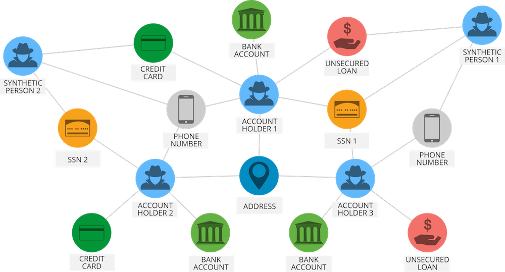
Network and IT Operations: Maps systems, devices, and dependencies to predict outage impacts or plan upgrades.
Personalized Recommendation: Enables context-aware recommendations by combining purchase history and social relationships.
Knowledge Graph: Used for enterprise knowledge management — linking people, documents, and systems to improve discovery.
Neo4j shines wherever relationships matter more than individual records — offering a flexible, intuitive, and highly connected way to store and analyze data.
[Avg. reading time: 3 minutes]
Neo4J Terms
Instead of having rows and columns, it has nodes, edges, and properties. It is more suitable for specific big data and analytics applications than row and column databases or free-form JSON document databases for many use cases.
A graph database is used to represent relationships. The most common examples of this are the Facebook Friend and Like relationships.
| RDBMS (MySQL) | Neo4J |
|---|---|
| Rows | Nodes |
| Tables | Labels |
| Columns | Properties |
| Foreign Key | Relationships |
| SQL | CQL (Cypher Query Language) |
| create database | create database |
| show database | :dbs |
| use database | :use database |
| show tables | call db.labels() |
| # Comments | // Comments |
| SELECT * from table | Match (n) return n |
Protocols
bolt:// – for drivers (fastest, binary). Default Bolt port: 7687
http(s):// – for REST API access (simpler, but slower)
| Protocol | Description |
|---|---|
| Bolt | Binary protocol designed by Neo4j for high-performance client communication. Default port: 7687. |
| HTTP/HTTPS | RESTful interface for interacting with Neo4j using tools like curl or browsers. Ports: 7474 (HTTP), 7473 (HTTPS). |
[Avg. reading time: 2 minutes]
Software
Free Client Software
Container Version
create folders neo4j/data
cd neo4j
podman run \
  --name myneo -d \
  -p7474:7474 -p7687:7687 \
  --volume=$PWD/data:/data \
  -e NEO4J_AUTH=neo4j/admin123 \
  -e NEO4J_PLUGINS='["apoc"]' \
  -e "NEO4J_dbms_security_procedures_unrestricted=apoc.*" \
  -e "NEO4J_dbms_security_procedures_allowlist=apoc.*" \
  docker.io/library/neo4j
Visit http://localhost:7474
default username/pwd: neo4j/admin123
Cloud - Free Server Account
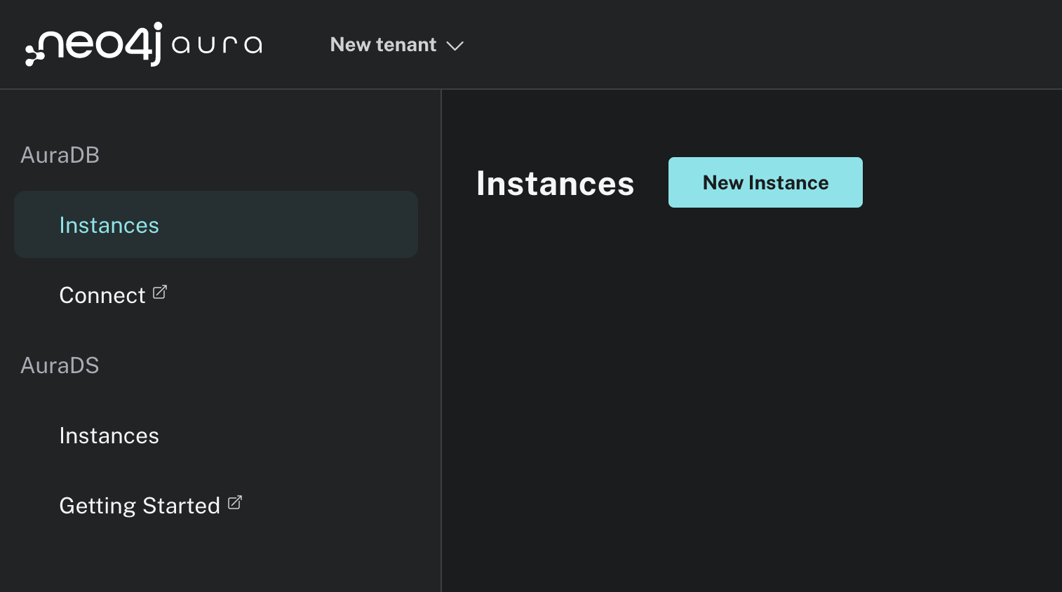
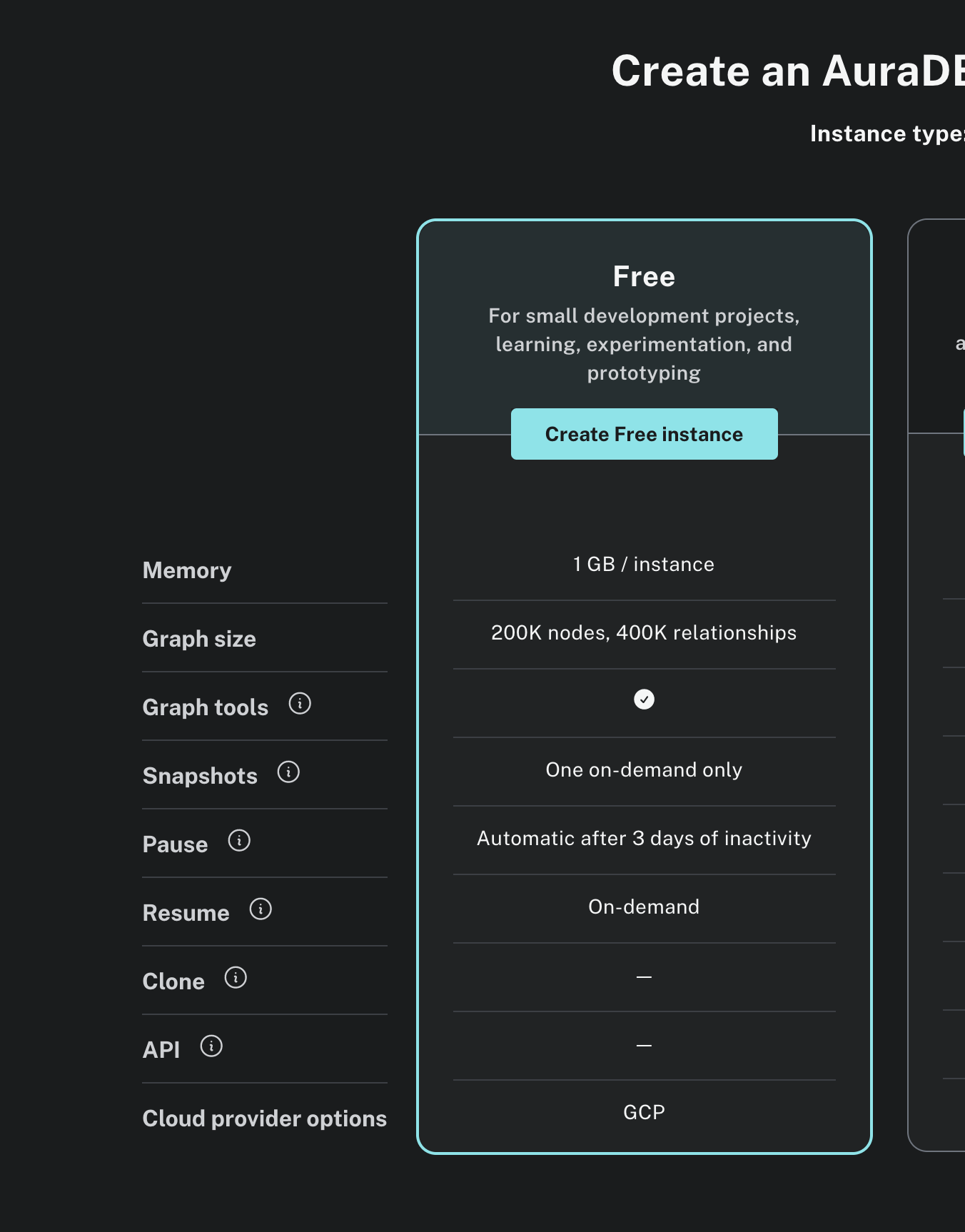
[Avg. reading time: 9 minutes]
Neo4J Components
Neo4j stores data as a property graph model, which consists of four main components.
- Nodes
- Labels
- Properties
- Relationships
Each component has a distinct role in representing and querying connected data.
In Neo4j, you don’t define tables or schemas ahead of time. You directly create nodes (data points) and optionally assign them labels and properties. The structure emerges dynamically from your data.
Node
// Create a single node
CREATE (n)

// Create two arbitrary nodes
CREATE (a), (b)

// View all nodes
MATCH (n) RETURN n;
In Cypher, (n) represents a node, and n is a variable you can use to refer to that node later.
Label
// Node with Label

create(n:Student)

match(y) return y
Label every node. Nodes without Labels are not useful.
A label defines the type or category of a node. You can think of it like a table name in SQL, but more flexible, a node can have multiple labels.
// To name a Node after Creation. Example ID=2 set Label to Building

match(n) where ID(n)=2 set n:somelabel

// To rename a Label

match(n) where ID(n)=2 set n:Building remove n:somelabel

match(n) return n
Example: 1 Node has 2 labels Person & Student.
CREATE (p:Person:Student {name:"Monica", major:"CS"});
Properties
create (n:Book{title:"The Sapiens", author:"Yuval Noah"});

create (n:Book{title:"Who Moved My Cheese", author:"Johnson M.D"});

MATCH (b:Book) RETURN b.title, b.author;

match(t) return t
Relationships
Create relationships.
Create a relationship between the existing nodes.
Create a relationship with labels and properties.
CREATE (node1)-[:RelationshipType]->(node2)
CREATE (a:Person {name:"Rachel"})-[:FRIENDS_WITH]->(b:Person {name:"Ross"});
MATCH (p:Person)-[r]->(f:Person) RETURN p, r, f;
EXPLAIN provides the execution plan for the query without actually running it. This allows you to understand how Neo4j will execute your query (e.g., which indexes it might use) and see if there are any inefficiencies in your Cypher.
EXPLAIN MATCH (p:Person)-[r]->(f:Person) RETURN p, r, f;
PROFILE executes the query and gives you a detailed execution plan along with runtime statistics. It shows the actual execution steps taken by the database, including how many records were passed through each step, making it more comprehensive than EXPLAIN.
PROFILE MATCH (p:Person)-[r]->(f:Person) RETURN p, r, f;
| Aspect | EXPLAIN | PROFILE |
|---|---|---|
| Execution | Does not run the query | Runs the query |
| Performance Stats | No | Yes |
| Use Case | Query plan analysis (safe, no data changes) | Actual performance analysis |
| Impact | Low (no data fetching or mutation) | Potentially high, especially on large datasets |
Maintenance Commands
Detach and Delete all nodes
MATCH (n) DETACH DELETE n;
Delete all relationships
MATCH ()-[r]-() DELETE r;
Update all nodes
MATCH (n) SET n.active = true;
[Avg. reading time: 2 minutes]
Hello World
It's Hello World time.
This query creates two nodes (Database and Message) and a relationship (SAYS) - your first connected graph in Neo4j.
CREATE (d:Database {name:"Neo4j"})-[r:SAYS]->(m:Message {name:"Hello World!"})
RETURN d,m r;
- d,m: Nodes
- Database, Message: Labels
- r: Relation
Neo4j → SAYS → Hello World!
Returns DB Version
To check the running Neo4j instance version:
CALL dbms.components()
YIELD name, versions, edition
RETURN name, versions[0], edition;
[Avg. reading time: 1 minute]
Examples
- Mysql Neo4j
- Sample Transactions
- Sample
- Create Nodes
- Update Nodes
- Relation
- Putting it all-together
- Commonly Used Functions
- Data Profiling
- Queries
- Load CSV into Neo4J
- Fraud Detection
- Python Scripts
[Avg. reading time: 5 minutes]
MySQL vs Neo4J
MySQL Tables
create table customer (id int,name varchar(100));
insert into customer values (1, 'Rachel');
create table creditcard (id int, number varchar(16));
insert into creditcard values (101, '1234567890123456');
create table merchant (id int, name varchar(100));
insert into merchant values (1001, 'Macys');
Set Relation
create table customer_creditcard (id int, cust_id int, cc_id int)
insert into customer_creditcard values (999, 1,101)
create table transaction (id int, customer_cc_id int, amount float, ts datetime);
insert into transaction(111, 999, 100.00, '2023-01-01 11:23:34')
erDiagram
    CUSTOMER {
        int id
        varchar name
    }
    CREDITCARD {
        int id
        varchar number
    }
    MERCHANT {
        int id
        varchar name
    }
    CUSTOMER_CREDITCARD {
        int id
        int cust_id
        int cc_id
    }
    TRANSACTION {
        int id
        int customer_cc_id
        float amount
        datetime ts
    }

    CUSTOMER ||--o{ CUSTOMER_CREDITCARD : "has"
    CREDITCARD ||--o{ CUSTOMER_CREDITCARD : "has"
    CUSTOMER_CREDITCARD ||--o{ TRANSACTION : "has"
Neo4J
Clear all nodes
match(n) detach delete n
CREATE (rachel:Customer {name: 'Rachel'})

CREATE (card1:CreditCard {number: '1234567890123456'})

CREATE (macys:Merchant {name: 'Macys'})

CREATE (rachel)-[:OWNS]->(card1)

CREATE (tx1:Transaction {amount: 100, timestamp: datetime()})

CREATE (card1)-[:USED_IN]->(tx1)-[:MADE_AT]->(macys)
graph TD
    rachel["Customer: Rachel"]
    card1["CreditCard: 1234567890123456"]
    macys["Merchant: Macys"]
    tx1["Transaction: Amount 100, Timestamp datetime()"]

    rachel -->|OWNS| card1
    card1 -->|USED_IN| tx1
    tx1 -->|MADE_AT| macys
[Avg. reading time: 20 minutes]
Sample Transactions
Run them individual blocks, see what went wrong and then run them in bulk to see the difference.
// Create sample nodes
CREATE (rachel:Customer {name: 'Rachel'})
CREATE (ross:Customer {name: 'Ross'})
CREATE (monica:Customer {name: 'Monica'})
CREATE (chandler:Customer {name: 'Chandler'})
CREATE (joey:Customer {name: 'Joey'})
CREATE (phoebe:Customer {name: 'Phoebe'})
CREATE (card1:CreditCard {number: '1234567890123456'})
CREATE (card2:CreditCard {number: '9876543210987654'})
CREATE (card3:CreditCard {number: '2345678901234567'})
CREATE (card4:CreditCard {number: '7890123456789012'})
CREATE (card5:CreditCard {number: '3456789012345678'})
CREATE (card6:CreditCard {number: '6789012345678901'})
CREATE (macys:Merchant {name: 'Macys'})
CREATE (officeDepot:Merchant {name: 'Office Depot'})
CREATE (centralPerk:Merchant {name: 'Central Perk'})
CREATE (pizzaHut:Merchant {name: 'Pizza Hut'})
CREATE (bloomingdales:Merchant {name: 'Bloomingdales'})
// Create relationships
CREATE (rachel)-[:OWNS]->(card1)
CREATE (ross)-[:OWNS]->(card2)
CREATE (monica)-[:OWNS]->(card3)
CREATE (chandler)-[:OWNS]->(card4)
CREATE (joey)-[:OWNS]->(card5)
CREATE (phoebe)-[:OWNS]->(card6)
// Create sample transactions
CREATE (tx1:Transaction {amount: 100, timestamp: datetime()})
CREATE (tx2:Transaction {amount: 200, timestamp: datetime()})
CREATE (tx3:Transaction {amount: 50, timestamp: datetime()})
CREATE (tx4:Transaction {amount: 300, timestamp: datetime()})
CREATE (tx5:Transaction {amount: 75, timestamp: datetime()})
CREATE (tx6:Transaction {amount: 120, timestamp: datetime()})
CREATE (tx7:Transaction {amount: 500, timestamp: datetime()})
CREATE (tx8:Transaction {amount: 40, timestamp: datetime()})
CREATE (tx9:Transaction {amount: 250, timestamp: datetime()})
CREATE (tx10:Transaction {amount: 80, timestamp: datetime()})
CREATE (card1)-[:USED_IN]->(tx1)-[:MADE_AT]->(macys)
CREATE (card1)-[:USED_IN]->(tx2)-[:MADE_AT]->(officeDepot)
CREATE (card2)-[:USED_IN]->(tx3)-[:MADE_AT]->(macys)
CREATE (card2)-[:USED_IN]->(tx4)-[:MADE_AT]->(officeDepot)
CREATE (card3)-[:USED_IN]->(tx5)-[:MADE_AT]->(centralPerk)
CREATE (card3)-[:USED_IN]->(tx6)-[:MADE_AT]->(bloomingdales)
CREATE (card4)-[:USED_IN]->(tx7)-[:MADE_AT]->(macys)
CREATE (card5)-[:USED_IN]->(tx8)-[:MADE_AT]->(pizzaHut)
CREATE (card5)-[:USED_IN]->(tx9)-[:MADE_AT]->(macys)
CREATE (card6)-[:USED_IN]->(tx10)-[:MADE_AT]->(centralPerk)
match(t)-[r]->(y) return t,r,y
Delete All the Nodes
match (t) detach delete t;

CREATE (rachel:Customer {name: 'Rachel'})
CREATE (ross:Customer {name: 'Ross'})
CREATE (monica:Customer {name: 'Monica'})
CREATE (chandler:Customer {name: 'Chandler'})
CREATE (joey:Customer {name: 'Joey'})
CREATE (phoebe:Customer {name: 'Phoebe'})

CREATE (card1:CreditCard {number: '1234567890123456'})
CREATE (card2:CreditCard {number: '9876543210987654'})
CREATE (card3:CreditCard {number: '2345678901234567'})
CREATE (card4:CreditCard {number: '7890123456789012'})
CREATE (card5:CreditCard {number: '3456789012345678'})
CREATE (card6:CreditCard {number: '6789012345678901'})

CREATE (macys:Merchant {name: 'Macys', location: 'New York'})
CREATE (officeDepot:Merchant {name: 'Office Depot', location: 'New Jersey'})
CREATE (centralPerk:Merchant {name: 'Central Perk', location: 'New York'})
CREATE (pizzaHut:Merchant {name: 'Pizza Hut', location: 'Chicago'})
CREATE (bloomingdales:Merchant {name: 'Bloomingdales', location: 'Boston'})

CREATE (rachel)-[:OWNS]->(card1)
CREATE (ross)-[:OWNS]->(card2)
CREATE (monica)-[:OWNS]->(card3)
CREATE (chandler)-[:OWNS]->(card4)
CREATE (joey)-[:OWNS]->(card5)
CREATE (phoebe)-[:OWNS]->(card6)


CREATE (tx1:Transaction {amount: 100, timestamp: datetime("2025-04-08T08:00:00")})
CREATE (tx2:Transaction {amount: 200, timestamp: datetime("2025-04-08T08:03:00")})
CREATE (tx3:Transaction {amount: 50, timestamp: datetime("2025-04-08T08:00:10")})
CREATE (tx4:Transaction {amount: 300, timestamp: datetime("2025-04-08T08:05:00")})
CREATE (tx5:Transaction {amount: 75, timestamp: datetime("2025-04-08T09:00:00")})
CREATE (tx6:Transaction {amount: 120, timestamp: datetime("2025-04-08T09:10:00")})
CREATE (tx7:Transaction {amount: 500, timestamp: datetime("2025-04-08T10:00:00")})
CREATE (tx8:Transaction {amount: 40, timestamp: datetime("2025-04-08T10:10:00")})
CREATE (tx9:Transaction {amount: 250, timestamp: datetime("2025-04-08T10:12:00")})
CREATE (tx10:Transaction {amount: 80, timestamp: datetime("2025-04-08T11:00:00")})

CREATE (card1)-[:USED_IN]->(tx1)-[:MADE_AT]->(macys)
CREATE (card1)-[:USED_IN]->(tx2)-[:MADE_AT]->(officeDepot)
CREATE (card2)-[:USED_IN]->(tx3)-[:MADE_AT]->(macys)
CREATE (card2)-[:USED_IN]->(tx4)-[:MADE_AT]->(officeDepot)
CREATE (card3)-[:USED_IN]->(tx5)-[:MADE_AT]->(centralPerk)
CREATE (card3)-[:USED_IN]->(tx6)-[:MADE_AT]->(bloomingdales)
CREATE (card4)-[:USED_IN]->(tx7)-[:MADE_AT]->(macys)
CREATE (card5)-[:USED_IN]->(tx8)-[:MADE_AT]->(pizzaHut)
CREATE (card5)-[:USED_IN]->(tx9)-[:MADE_AT]->(macys)
CREATE (card6)-[:USED_IN]->(tx10)-[:MADE_AT]->(centralPerk)
match(t)-[r]->(y) return t,r,y
Find all customers
MATCH (c:Customer)
RETURN c.name
Find all transactions made at Macys
MATCH (tx:Transaction)-[:MADE_AT]->(m:Merchant)
WHERE m.name = 'Macys'
RETURN tx.amount, tx.timestamp
Find all credit cards owned by Ross
MATCH (ross:Customer {name: 'Ross'})-[:OWNS]->(card:CreditCard)
RETURN card.number
Find the customer who made a specific transaction for 120
MATCH (c:Customer)-[:OWNS]->(card:CreditCard)-[:USED_IN]->(tx:Transaction)
WHERE tx.amount = 120
RETURN c.name
Find the merchants where Monica made transactions
MATCH (monica:Customer {name: 'Monica'})-[:OWNS]->(card:CreditCard)-[:USED_IN]->(tx:Transaction)-[:MADE_AT]->(m:Merchant)
RETURN DISTINCT m.name
Find the total amount spent by Chandler at Macys
MATCH (chandler:Customer {name: 'Chandler'})-[:OWNS]->(card:CreditCard)-[:USED_IN]->(tx:Transaction)-[:MADE_AT]->(macys:Merchant {name: 'Macys'})
RETURN SUM(tx.amount) AS total_spent
Fraud Transactions
- High-value transactions
MATCH (c:Customer)-[:OWNS]->(cc:CreditCard)-[:USED_IN]->(tx:Transaction)
WHERE tx.amount > 400
RETURN c.name AS customer, cc.number AS card, tx.amount AS amount, tx.timestamp AS time, 'FRAUD' AS flagged_reason
Logical View
apoc - Awesome procedures on Cypher
MATCH (c:Customer)-[:OWNS]->(cc:CreditCard)-[:USED_IN]->(tx:Transaction)
WHERE tx.amount > 400
CALL apoc.create.vRelationship(c, "FRAUD", {}, tx) YIELD rel
RETURN c, rel, tx
Making an Update
MATCH (c:Customer)-[:OWNS]->(cc:CreditCard)-[:USED_IN]->(tx:Transaction)
WHERE tx.amount > 400
MERGE (c)-[:FRAUD]->(tx)
RETURN c,tx
- Quick back-to-back use of same card at different merchants
MATCH (c:Customer)-[:OWNS]->(cc:CreditCard)-[:USED_IN]->(t1:Transaction)-[:MADE_AT]->(m1:Merchant),
      (cc)-[:USED_IN]->(t2:Transaction)-[:MADE_AT]->(m2:Merchant)
WHERE m1.name <> m2.name
  AND abs(datetime(t1.timestamp).epochSeconds - datetime(t2.timestamp).epochSeconds) < 300
  AND t1 <> t2
RETURN
  c.name AS Customer,
  cc.number AS CardNumber,
  t1.timestamp AS FirstTxTime,
  m1.name AS FirstMerchant,
  t2.timestamp AS SecondTxTime,
  m2.name AS SecondMerchant,
  'Geo-impossible usage (too fast)' AS FraudReason
MATCH (c:Customer)-[:OWNS]->(cc:CreditCard)-[:USED_IN]->(t1:Transaction)-[:MADE_AT]->(m1:Merchant),
      (cc)-[:USED_IN]->(t2:Transaction)-[:MADE_AT]->(m2:Merchant)
WHERE m1.name <> m2.name
  AND abs(datetime(t1.timestamp).epochSeconds - datetime(t2.timestamp).epochSeconds) < 300
  AND t1 <> t2
CALL apoc.create.vRelationship(c, "FRAUD", {reason: "Geo-impossible usage"}, t2) YIELD rel
RETURN c, rel, t1, m1, t2, m2
MATCH (c:Customer)-[:OWNS]->(cc:CreditCard)-[:USED_IN]->(t1:Transaction)-[:MADE_AT]->(m1:Merchant),
      (cc)-[:USED_IN]->(t2:Transaction)-[:MADE_AT]->(m2:Merchant)
WHERE m1.name <> m2.name
  AND abs(datetime(t1.timestamp).epochSeconds - datetime(t2.timestamp).epochSeconds) < 300
MERGE (c)-[:FRAUD]->(t2)
RETURN c,t1,m1,t2,m2
- List All fraud transactions
MATCH (c:Customer)-[:FRAUD]->(t:Transaction)
RETURN c.name AS Fraudster, t.amount, t.timestamp
- List all Genuine Transactions
MATCH (c:Customer)-[:OWNS]->(cc:CreditCard)-[:USED_IN]->(tx:Transaction)
WHERE NOT (c)-[:FRAUD]->(tx)
RETURN c.name AS Customer, cc.number AS CardNumber, tx.amount AS Amount, tx.timestamp AS Time
ORDER BY tx.timestamp
Better Use Case
[Avg. reading time: 0 minutes]
Sample
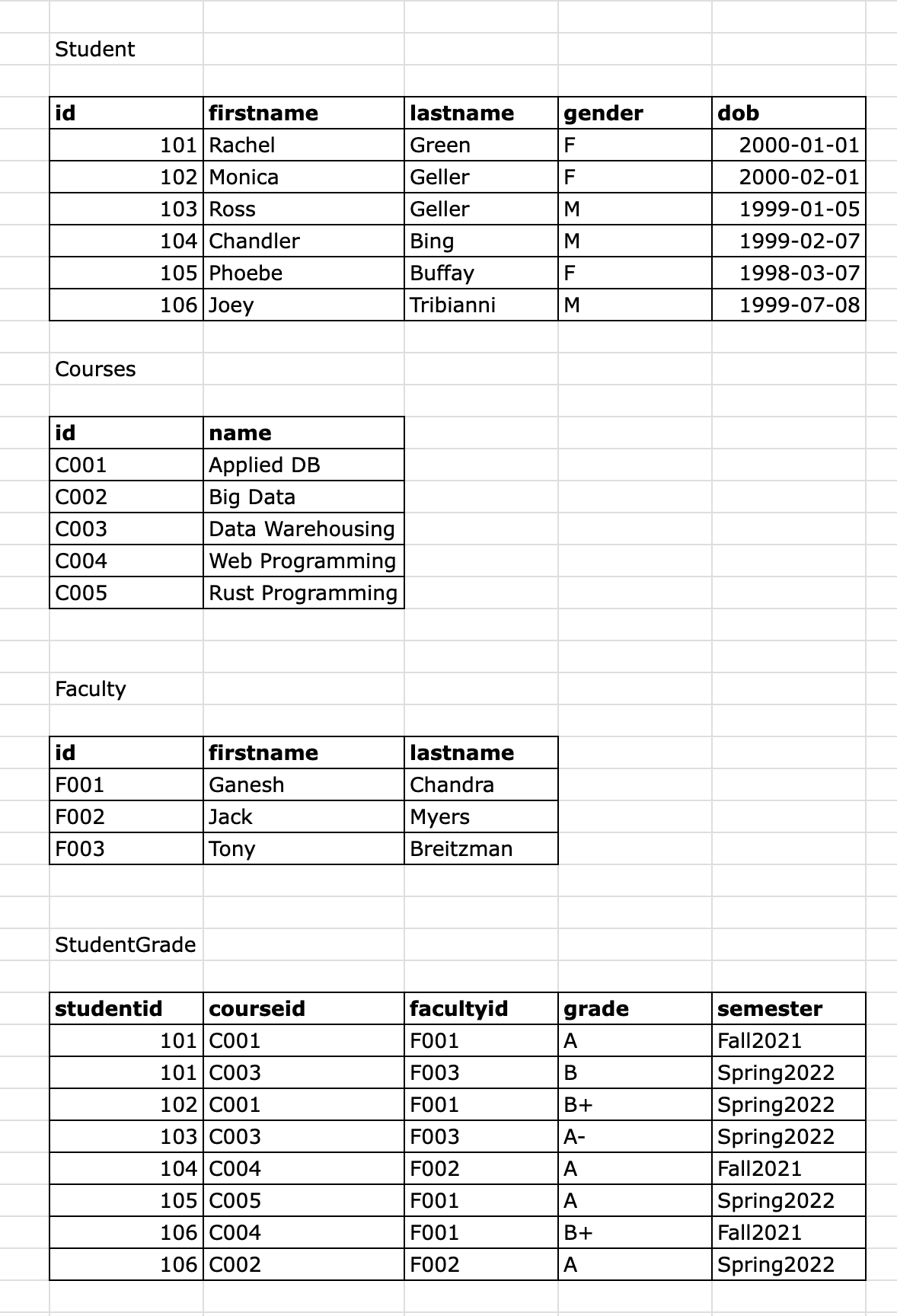
[Avg. reading time: 6 minutes]
Create Nodes
// delete all existing nodes

match (n) detach delete n;

// create new nodes

create (n:Student{id:101,firstname:"Rachel",lastname:"Green",gender:"F",dob:"2000-01-01"});
create (n:Student{id:102,firstname:"Monica",lastname:"Geller",gender:"F",dob:"2000-02-01"});
create (n:Student{id:103,firstname:"Ross",lastname:"Green",gender:"M",dob:"1999-01-05"});
create (n:Student{id:104,firstname:"Chandler",lastname:"Bing",gender:"M",dob:"1999-02-07"});
create (n:Student{id:105,firstname:"Phoebe",lastname:"Buffay",gender:"F",dob:"1998-03-07"});
create (n:Student{id:106,firstname:"Joey",lastname:"Tribianni",gender:"M",dob:"1999-07-08"});
create (n:Student{id:107,firstname:"Janice",gender:"F",dob:"2000-07-08"});

match(y) return y
Constraints
CREATE CONSTRAINT cons_stuid_notnull IF NOT EXISTS FOR (n:Student) REQUIRE n.id IS NOT NULL

CREATE CONSTRAINT cons_stuid_unique IF NOT EXISTS FOR (n:Student) REQUIRE n.id IS UNIQUE

show constraints

drop constraint cons_stuid_unique
Create another student without an ID
create (n:Student{firstname:"Gunther",gender:"M",dob:"1995-07-08"});
Error??
create (n:Student{id:108,firstname:"Gunther",gender:"M",dob:"1995-07-08"});
// create with ID

create (n:Student{id:108,firstname:"Gunther",gender:"M",dob:"1995-07-08"});

// try again to test for Unique

create (n:Student{id:108,firstname:"Gunther",gender:"M",dob:"1995-07-08"});
create (t:Course{id:"C001",name:"Applied DB"});
create (t:Course{id:"C002",name:"Big Data"});
create (t:Course{id:"C003",name:"Data Warehousing"});
create (t:Course{id:"C004",name:"Web Programming"});
create (t:Course{id:"C005",name:"Rust Programming"});
create (z:Faculty{id:"F001",firstname:"Ganesh",lastname:"Chandra"});
create (z:Faculty{id:"F002",firstname:"Jack",lastname:"Myers"});
create (z:Faculty{id:"F003",firstname:"Tony",lastname:"Brietzman"});
View all nodes
match (t) return t
[Avg. reading time: 1 minute]
Update Nodes
// Update existing property
MATCH (a:Student) WHERE a.id = 103
set a.lastname='Geller';
// Add new property
MATCH (n {firstname: 'Janice' })
SET n.favouriteline = 'Oh My God'
RETURN n.firstname, n.favouriteline;
Indexes
CREATE INDEX student_name FOR (n:Student) ON (n.firstname)
SHOW INDEXES
DROP INDEX student_name
[Avg. reading time: 7 minutes]
Relation
CREATE - Always creates a new relationship, regardless of whether it already exists. Creates a duplicate if already exists.
MERGE - Creates if not exists. Idempotent.
// Create a Relation
MATCH (a:Student),(b:Course) WHERE a.firstname = 'Rachel' AND b.id = 'C001'
CREATE (a)-[:TAKING]->(b);
MATCH (a:Student),(b:Course) WHERE a.firstname = 'Rachel' AND b.id = 'C003'
MERGE (a)-[:TAKING]->(b);
//Relation Set wrong way
MATCH (a:Student),(b:Course) WHERE a.firstname = 'Monica' AND b.id = 'C001'
MERGE (a)<-[:TAKING]-(b);
// Delete the relation
MATCH (a:Student)<-[r:TAKING]-(b:Course) WHERE a.firstname = 'Monica' AND b.id = 'C001' DELETE r;
// Recreat the relation
MATCH (a:Student),(b:Course) WHERE a.firstname = 'Monica' AND b.id = 'C001'
MERGE (a)-[:TAKING {grade:"B+"}]->(b);
//
MATCH (a:Student),(b:Course),(c:Faculty) WHERE a.id = 101 AND b.id = 'C003' AND c.id='F003'
MERGE (c)-[:TEACHING]->(b)<-[:TAKING {grade:"A-",semester:"Spring2022"}]-(a);
// this MERGEs duplicate link between Tony and DW
MATCH (a:Student),(b:Course),(c:Faculty) WHERE a.id = 103 AND b.id = 'C003' AND c.id='F003'
MERGE (c)-[:TEACHING]->(b)<-[:TAKING {grade:"A-",semester:"Spring2022"}]-(a);
// This way avoids it but it also doesnt MERGE Ross and DW
MATCH (a:Student),(b:Course),(c:Faculty) WHERE a.id = 103 AND b.id = 'C003' AND c.id='F003' AND NOT (c)-[:TEACHING]->(b)
MERGE (c)-[:TEACHING]->(b)<-[:TAKING {grade:"A-",semester:"Spring2022"}]-(a);
MATCH (a:Student),(b:Course) WHERE a.id = 103 AND b.id = 'C003'
MERGE (a)-[:TAKING {grade:"A-"}]->(b);
MATCH (a:Student),(b:Course) WHERE a.id = 104 AND b.id = 'C004'
MERGE (a)-[:TAKING {grade:"A"}]->(b);
MATCH (a:Student),(b:Course) WHERE a.id = 105 AND b.id = 'C005'
MERGE (a)-[:TAKING {grade:"A"}]->(b);
MATCH (a:Student),(b:Course),(c:Faculty) WHERE a.id = 106 AND b.id = 'C004' AND c.id='F001'
MERGE (a)-[:TAKING {grade:"B+"}]->(b)<-[:TEACHING]-(c);
MATCH (a:Student),(b:Course),(c:Faculty) WHERE a.id = 106 AND b.id = 'C002' AND c.id='F002'
MERGE (a)-[:TAKING {grade:"A-"}]->(b)<-[:TEACHING]-(c);
MATCH (a:Student{firstname:"Joey"})-[r]-(b:Course{id:"C002"})
SET r.grade = "A", r.semester="Spring2022"
MATCH (a:Student{firstname:"Monica"})-[r]-(b:Course{id:"C001"})
SET r.grade = "B+"
MATCH (a:Student),(b:Course),(c:Faculty) WHERE a.id = 101 AND b.id = 'C001' AND c.id='F001'
MERGE (c)-[:TEACHING]->(b);
MATCH (a:Student),(b:Course),(c:Faculty) WHERE a.id = 103 AND b.id = 'C003' AND c.id='F003'
MERGE (c)-[:TEACHING]->(b);
MATCH (a:Student)<-[r:TAKING]-(b:Course) WHERE a.firstname = 'Ross' AND b.id = 'C003' DELETE r;
[Avg. reading time: 16 minutes]
Putting it all together
match (n) detach delete n;
create (n:Student{id:101,firstname:"Rachel",lastname:"Green",gender:"F",dob:"2000-01-01"});
create (n:Student{id:102,firstname:"Monica",lastname:"Geller",gender:"F",dob:"2000-02-01"});
create (n:Student{id:103,firstname:"Ross",lastname:"Geller",gender:"M",dob:"1999-01-05"});
create (n:Student{id:104,firstname:"Chandler",lastname:"Bing",gender:"M",dob:"1999-02-07"});
create (n:Student{id:105,firstname:"Phoebe",lastname:"Buffay",gender:"F",dob:"1998-03-07"});
create (n:Student{id:106,firstname:"Joey",lastname:"Tribianni",gender:"M",dob:"1999-07-08"});
create (n:Student{id:107,firstname:"Janice",gender:"F",dob:"2000-07-08"});
CREATE CONSTRAINT cons_stuid_notnull IF NOT EXISTS FOR (n:Student) REQUIRE n.id IS NOT NULL;
CREATE CONSTRAINT cons_stuid_unique IF NOT EXISTS FOR (n:Student) REQUIRE n.id IS UNIQUE;
create (n:Student{id:108,firstname:"Gunther",gender:"M",dob:"1995-07-08"});
create (t:Course{id:"C001",name:"Applied DB"});
create (t:Course{id:"C002",name:"Big Data"});
create (t:Course{id:"C003",name:"Data Warehousing"});
create (t:Course{id:"C004",name:"Web Programming"});
create (t:Course{id:"C005",name:"Rust Programming"});
create (z:Faculty{id:"F001",firstname:"Ganesh",lastname:"Chandra"});
create (z:Faculty{id:"F002",firstname:"Jack",lastname:"Myers"});
create (z:Faculty{id:"F003",firstname:"Tony",lastname:"Brietzman"});
MATCH (a:Student),(b:Course),(c:Faculty) WHERE a.id = 101 AND b.id = 'C001' AND c.id='F001'
MERGE (c)-[:TEACHING]->(b)
MERGE (b)<-[:TAKING {grade:"A",semester:"Fall2021"}]-(a);
MATCH (a:Student),(b:Course),(c:Faculty) WHERE a.id = 101 AND b.id = 'C003' AND c.id='F003'
MERGE (c)-[:TEACHING]->(b)
MERGE (b)<-[:TAKING {grade:"B",semester:"Spring2022"}]-(a);
MATCH (a:Student),(b:Course),(c:Faculty) WHERE a.id = 102 AND b.id = 'C001' AND c.id='F001'
MERGE (c)-[:TEACHING]->(b)
MERGE (b)<-[:TAKING {grade:"B+",semester:"Spring2022"}]-(a);
MATCH (a:Student),(b:Course),(c:Faculty) WHERE a.id = 101 AND b.id = 'C003' AND c.id='F003'
MERGE (c)-[:TEACHING]->(b)
MERGE (b)<-[:TAKING {grade:"B",semester:"Spring2022"}]-(a);
MATCH (a:Student),(b:Course),(c:Faculty) WHERE a.id = 103 AND b.id = 'C003' AND c.id='F003'
MERGE (c)-[:TEACHING]->(b)
MERGE (b)<-[:TAKING {grade:"A-",semester:"Spring2022"}]-(a);
MATCH (a:Student),(b:Course),(c:Faculty) WHERE a.id = 104 AND b.id = 'C004' AND c.id='F002'
MERGE (c)-[:TEACHING]->(b)
MERGE (b)<-[:TAKING {grade:"A",semester:"Fall2021"}]-(a);
MATCH (a:Student),(b:Course),(c:Faculty) WHERE a.id = 105 AND b.id = 'C005' AND c.id='F001'
MERGE (c)-[:TEACHING]->(b)
MERGE (b)<-[:TAKING {grade:"A",semester:"Spring2022"}]-(a);
MATCH (a:Student),(b:Course),(c:Faculty) WHERE a.id = 106 AND b.id = 'C004' AND c.id='F001'
MERGE (c)-[:TEACHING]->(b)
MERGE (b)<-[:TAKING {grade:"B+",semester:"Fall2021"}]-(a);
MATCH (a:Student),(b:Course),(c:Faculty) WHERE a.id = 106 AND b.id = 'C002' AND c.id='F002'
MERGE (c)-[:TEACHING]->(b)
MERGE (b)<-[:TAKING {grade:"A",semester:"Spring2022"}]-(a);
MATCH (a:Student),(b:Course),(c:Faculty) WHERE a.id = 107 AND b.id = 'C005' AND c.id='F001'
MERGE (c)-[:TEACHING]->(b)
MERGE (b)<-[:TAKING {grade:"A",semester:"Fall2021"}]-(a);
Queries
- Retrieve All Students
MATCH (n:Student) RETURN n;
- Find a Specific Student by ID
MATCH (n:Student {id:101}) RETURN n;
3. List All Courses
MATCH (n:Course) RETURN n.name;
4. Find Students Taking a Specific Course
MATCH (s:Student)-[:TAKING]->(c:Course {id:"C001"})
RETURN s.firstname, s.lastname;
5. List Courses Taught by a Specific Faculty
MATCH (f:Faculty {id:"F001"})-[:TEACHING]->(c:Course)
RETURN f.firstname, f.lastname, collect(c.name) AS Courses;
6. Find Students and Their Grades for a Specific Course
MATCH (s:Student)-[r:TAKING]->(c:Course {id:"C002"})
RETURN s.firstname, s.lastname, r.grade;
7. Find Average Grade for Each Course
MATCH (s:Student)-[r:TAKING]->(c:Course)
RETURN c.name, avg(toFloat(r.grade)) AS AverageGrade
ORDER BY AverageGrade DESC;
8. Identify Students Taking Courses with a Specific Faculty
MATCH (s:Student)-[:TAKING]->(c:Course)<-[:TEACHING]-(f:Faculty {id:"F001"})
RETURN s.firstname, s.lastname, collect(c.name) AS Courses;
9. Create a Friendship Relationship Between Students
MATCH (s1:Student {id:101}), (s2:Student {id:102})
MERGE (s1)-[:FRIENDS_WITH]->(s2);
Creates a "FRIENDS_WITH" relationship between two students.
10. Find Students and the Number of Courses They Are Taking
MATCH (s:Student)-[:TAKING]->(c:Course)
RETURN s.firstname, s.lastname, count(c) AS CoursesTaken
ORDER BY CoursesTaken DESC;
Counts how many courses each student is taking.
11. Find the Most Popular Course
MATCH (s:Student)-[:TAKING]->(c:Course)
WITH c, count(s) AS StudentCount
ORDER BY StudentCount DESC
LIMIT 1
RETURN c.name, StudentCount;
12. Students and Their Friends Taking the Same Course
MATCH (s:Student)-[:FRIENDS_WITH]->(friend:Student)-[:TAKING]->(course:Course), (s)-[:TAKING]->(course)
RETURN s.firstname, friend.firstname, course.name;
13. Search by Semester & Grade
MATCH (s:Student)-[r:TAKING]->(c:Course)
WHERE r.semester = "Spring2022"
AND r.grade =~ "[A-C].*|D+"
RETURN s.id AS StudentID, s.firstname AS FirstName, s.lastname AS LastName, c.id AS CourseID, c.name AS CourseName, r.grade AS Grade
14. Show all connected nodes for a given node (upto 4 levels)
MATCH (ross:Student {firstname:"Ross"})-[*1..4]-(connectedNodes)
RETURN ross, connectedNodes;
15. Show all connected nodes.
MATCH (ross:Student {firstname:"Ross"})-[*1..]-(connectedNodes)
RETURN ross, connectedNodes;
[Avg. reading time: 7 minutes]
Commonly used Functions
String Functions
match (a) return toUpper(a.firstname);
RETURN left('hello', 3)
RETURN lTrim(' hello')
RETURN replace("hello", "l", "w")
RETURN reverse('hello')
RETURN substring('hello', 1, 3), substring('hello', 2)
RETURN toString(11.5),
toString('already a string'),
toString(true),
toString(date({year:1984, month:10, day:11})) AS dateString,
toString(datetime({year:1984, month:10, day:11, hour:12, minute:31, second:14, millisecond: 341, timezone: 'Europe/Stockholm'})) AS datetimeString,
toString(duration({minutes: 12, seconds: -60})) AS durationString
Aggregation Functions
-
COUNT: Counts the number of items.
MATCH (n:Student) RETURN COUNT(n); -
MAX and MIN: Find the maximum or minimum of a set of values.
MATCH (n:Student)-[r:TAKING]->(c) RETURN MAX(r.grade), MIN(r.grade);
Date and Time Functions
-
date(): Creates a date from a string or a map.
RETURN date('2024-03-20'); -
datetime(): Creates a datetime from a string or a map.
RETURN datetime('2024-03-20T12:00:00'); -
duration.between(): Calculates the duration between two temporal values.
RETURN duration.between(date('1984-10-11'), date('2024-03-20'));
List Functions
-
COLLECT: Aggregates values into a list.
MATCH (n:Student) RETURN COLLECT(n.firstname); -
SIZE: Returns the size of a list.
MATCH (n:Student) RETURN COLLECT(n.firstname), SIZE(COLLECT(n.firstname)); -
RANGE: Creates a list containing a sequence of integers.
RETURN RANGE(1, 10, 2);
Mathematical Functions
-
ABS: Returns the absolute value.
RETURN ABS(-42); -
ROUND, CEIL, FLOOR: Round numbers to the nearest integer, up, or down.
RETURN ROUND(3.14159), CEIL(3.14159), FLOOR(3.14159);
Logical Functions
-
COALESCE: Returns the first non-null value in a list of expressions.
RETURN COALESCE(NULL, 'first non-null', NULL);
Spatial Functions
-
point: Creates a point in a 2D space (or 3D if you add elevation) which can be used for spatial queries.
RETURN point({latitude: 37.4847, longitude: -122.148}) -
distance: Calculates the geodesic distance between two points in Meters. Cherryhill to Moorestown. Verify the result https://www.nhc.noaa.gov/gccalc.shtml
RETURN point.distance( point({latitude: 39.94, longitude: -75.01}), point({latitude: 39.97, longitude: -74.96}) ) / 1609.34 AS distanceInMiles -
apoc.coll.sort: Sorts a list.
RETURN apoc.coll.sort(['banana', 'apple', 'cherry']) -
apoc.map.merge: Merges two maps.
RETURN apoc.map.merge({name: 'Neo'}, {age: 23})
[Avg. reading time: 1 minute]
Data Profiling
// Count all nodes
MATCH (n) RETURN count(n)
// Count all relationships
MATCH ()-->() RETURN count(*);
// Display constraints and indexes
:schema
// List node labels
CALL db.labels()
// List relationship types
CALL db.relationshipTypes()
// What is related, and how
CALL db.schema.visualization()
[Avg. reading time: 3 minutes]
Queries
// Return all Gellers
match(b {lastname:"Geller"} ) return b
// get all the students who are taking "Applied DB" course
MATCH (m:Student)-[:TAKING]->(k:Course{name:"Applied DB"}) return m,k
// get all courses taught by Ganesh
MATCH (m:Faculty{firstname:"Ganesh"})-[:TEACHING]->(k) return m,k
// get all students of Ganesh
MATCH (m:Faculty{firstname:"Ganesh"})-[:TEACHING]->(k:Course)<-[r1:TAKING]-(l:Student) return m,k,l
// Get all the faculty who are teaching Web Programming
MATCH (c:Course{name:"Web Programming"})<-[:TEACHING]-(f) return f
// Get all the faculty and students who are learning Web Programming
MATCH (c:Course{name:"Web Programming"})<-[:TEACHING]-(f), (c)<-[:TAKING]-(s:Student) return f,s
// returning LIST of values
MATCH (c:Course{name:"Web Programming"})<-[:TEACHING]-(f), (c)<-[:TAKING]-(s:Student) return collect(f.firstname)
MATCH (c:Course{name:"Web Programming"})<-[:TEACHING]-(f), (c)<-[:TAKING]-(s:Student) return collect(distinct f.firstname)
[Avg. reading time: 21 minutes]
Load CSV into Neo4J
APOC
APOC stands for "Awesome Procedures On Cypher". It is a popular library of user-defined procedures and functions for Neo4j, extending the functionality of the core database. APOC provides many utilities for data manipulation, graph algorithms, integration with external systems, and various helper functions that make working with Neo4j more powerful and convenient.
Key Features of APOC
Data Conversion:
Convert between different data types (e.g., dates, numbers, JSON). Parse and format dates easily.
Data Integration:
Import data from CSV, JSON, or external APIs. Export data to JSON, CSV, or other formats.
Graph Algorithms:
Perform advanced graph queries and algorithms not available in Cypher by default.
Utilities for Cypher Queries:
Run parallel queries, manage transactions, and work with lists, maps, or collections.
Improved Indexing and Search:
Help with text searches, schema indexing, and optimized lookups.
WITH Statement
The WITH clause in Neo4j serves multiple purposes. It allows you to chain parts of a query, pass results between stages, perform filtering and aggregation, and ensure that certain operations (like pagination or filtering) are done after aggregation.
Using WITH, you pass intermediate results from one stage to the next. Its like a pipeline manager.
Example
match(t) detach delete t;
CREATE (p1:Person {name: "Rachel"})
CREATE (p2:Person {name: "Ross"})
CREATE (p3:Person {name: "Chandler"})
CREATE (p4:Person {name: "Joey"})
CREATE (p5:Person {name: "Monica"})
CREATE (p6:Person {name: "Phoebe"})
CREATE (m1:Movie {title: "Inception", releaseDate: 2010, rating: 8.8})
CREATE (m2:Movie {title: "The Matrix", releaseDate: 1999, rating: 8.7})
CREATE (m3:Movie {title: "Interstellar", releaseDate: 2014, rating: 8.6})
CREATE (p1)-[:FRIEND]->(p2)
CREATE (p1)-[:FRIEND]->(p3)
CREATE (p2)-[:FRIEND]->(p4)
CREATE (p5)-[:FRIEND]->(p6)
CREATE (p1)-[:ACTED_IN]->(m1)
CREATE (p2)-[:ACTED_IN]->(m2)
CREATE (p3)-[:ACTED_IN]->(m3)
CREATE (p5)-[:ACTED_IN]->(m3)
CREATE (p1)-[:LIKES]->(m1)
CREATE (p2)-[:LIKES]->(m1)
CREATE (p3)-[:LIKES]->(m2)
CREATE (p4)-[:LIKES]->(m3)
CREATE (p4)-[:DISLIKES]->(m2)
CREATE (p6)-[:DISLIKES]->(m1)
View All
match(t)-[r]->(y) return t,r,y;
Count how many friends each person has and return only those with more than 1 friend.
MATCH (p:Person)-[:FRIEND]->(f:Person)
WITH p, count(f) AS friendCount
WHERE friendCount > 1
RETURN distinct p.name AS person, friendCount
Group people by the movie they both like
MATCH (m:Movie)<-[:LIKES]-(p:Person)
WITH m, collect(DISTINCT p.name) AS people
RETURN m.title AS movie, people
ORDER BY movie;
Convert String Date to Neo4J Date Format
WITH '10/30/2024' AS dateString
RETURN
apoc.date.parse(dateString, 'ms', 'MM/dd/yyyy') AS timestamp,
apoc.date.format(apoc.date.parse(dateString, 'ms', 'MM/dd/yyyy'), 'ms', 'yyyy-MM-dd') AS dataFormatInString,
date(apoc.date.format(apoc.date.parse(dateString, 'ms', 'MM/dd/yyyy'), 'ms', 'yyyy-MM-dd')) AS formattedDate
Talk about Epoch
Also print the datatype
WITH '10/30/2024' AS dateString
RETURN
apoc.date.parse(dateString, 'ms', 'MM/dd/yyyy') AS timestamp,
apoc.meta.cypher.type(apoc.date.parse(dateString, 'ms', 'MM/dd/yyyy')) AS timestampType,
apoc.date.format(apoc.date.parse(dateString, 'ms', 'MM/dd/yyyy'), 'ms', 'yyyy-MM-dd') AS dataFormatInString,
apoc.meta.cypher.type(apoc.date.format(apoc.date.parse(dateString, 'ms', 'MM/dd/yyyy'), 'ms', 'yyyy-MM-dd')) AS dataFormatType,
date(apoc.date.format(apoc.date.parse(dateString, 'ms', 'MM/dd/yyyy'), 'ms', 'yyyy-MM-dd')) AS formattedDate,
apoc.meta.cypher.type(date(apoc.date.format(apoc.date.parse(dateString, 'ms', 'MM/dd/yyyy'), 'ms', 'yyyy-MM-dd'))) AS formattedDateType
Load CSV into Neo4J
match(t) detach delete t;
LOAD CSV WITH HEADERS FROM 'https://raw.githubusercontent.com/gchandra10/filestorage/main/sales_100.csv' AS row
return row
LOAD CSV WITH HEADERS FROM 'https://raw.githubusercontent.com/gchandra10/filestorage/main/sales_100.csv' AS row
return row.Region,row.Country,row.`Order ID` as OrderID
LOAD CSV WITH HEADERS FROM 'https://raw.githubusercontent.com/gchandra10/filestorage/main/sales_100.csv' AS row
return row.Region,row.Country,toInteger(row.`Order ID`) as OrderID
LOAD CSV WITH HEADERS FROM 'https://raw.githubusercontent.com/gchandra10/filestorage/main/sales_100.csv' AS row
RETURN
row.`Order ID` AS orderId,
row.Country AS country,
row.Region AS region,
row.`Order Date` AS orderDate,
toInteger(row.UnitsSold) AS unitsSold,
toFloat(row.UnitPrice) AS unitPrice,
toFloat(row.TotalCost) AS totalCost,
toFloat(row.TotalProfit) AS totalProfit
LOAD CSV WITH HEADERS FROM 'https://raw.githubusercontent.com/gchandra10/filestorage/main/sales_100.csv' AS row
RETURN
row.`Order ID` AS orderId,
row.Country AS country,
row.Region AS region,
date(apoc.date.format(apoc.date.parse(row.`Order Date`, 'ms', 'MM/dd/yyyy'), 'ms', 'yyyy-MM-dd')) AS OrderDate,
toInteger(row.UnitsSold) AS unitsSold,
toFloat(row.UnitPrice) AS unitPrice,
toFloat(row.TotalCost) AS totalCost,
toFloat(row.TotalProfit) AS totalProfit
How to ingest this with Neo4J relations
-
One node per Order with properties for unitsSold, unitPrice, totalCost, totalProfit, OrderDate, country, region
- Fastest to ingest, lowest complexity
- weaker for joins, hierarchies, and reuse of country/region
-
Using top level Relations
- (Order)-[:IN_COUNTRY]->(Country), (Country)-[:IN_REGION]->(Region), (Order)-[:ON_DAY]->(Day)
- Best general-purpose pattern; supports drill-downs, reuse, and constraints
- Add uniqueness on orderId, country name, region name, date
-
Hierarchy-first model
- Region, Country; build the geography tree first (Country)-[:IN_REGION]->(Region)
- Attach Order nodes only to Country; roll-ups traverse Country→Region
Putting it all together
LOAD CSV WITH HEADERS FROM 'https://raw.githubusercontent.com/gchandra10/filestorage/main/sales_100.csv' AS row
MERGE (region:Region {name: row.Region})
MERGE (country:Country {name: row.Country})
MERGE (itemType:ItemType {name: row.`Item Type`})
MERGE (sale:Sale {
salesChannel: toString(row.`Sales Channel`),
orderPriority: toString(row.`Order Priority`),
orderDate: date(apoc.date.format(apoc.date.parse(row.`Order Date`, 'ms', 'MM/dd/yyyy'), 'ms', 'yyyy-MM-dd')),
orderId: toInteger(row.`Order ID`),
shipDate: date(apoc.date.format(apoc.date.parse(row.`Ship Date`, 'ms', 'MM/dd/yyyy'), 'ms', 'yyyy-MM-dd')),
unitsSold: toInteger(row.UnitsSold),
unitPrice: toFloat(row.UnitPrice),
unitCost: toFloat(row.UnitCost),
totalRevenue: toFloat(row.TotalRevenue),
totalCost: toFloat(row.TotalCost),
totalProfit: toFloat(row.TotalProfit)
})
MERGE (region)-[:CONTAINS]->(country)
MERGE (country)-[:SOLD_ITEM]->(sale)
MERGE (sale)-[:OF_TYPE {order_priority: sale.orderPriority}]->(itemType)
Avg Profit per Region
MATCH (r:Region)-[:CONTAINS]->(:Country)-[:SOLD_ITEM]->(s:Sale)
WITH r, sum(s.totalProfit) AS profit, sum(s.totalRevenue) AS revenue
RETURN r.name AS region, round(profit / revenue * 100,2) AS marginPercent
ORDER BY marginPercent DESC;
Return number of units sold by Region, Country
match (r:Region)-[:CONTAINS]->(c:Country)-[:SOLD_ITEM]->(s:Sale) return r.name, c.name, count(s.unitsSold) as cnt
Return number of units sold by Region, Country where count > 1
MATCH (r:Region)-[:CONTAINS]->(c:Country)-[:SOLD_ITEM]->(s:Sale)
WITH r.name AS regionName, c.name AS countryName, count(s) AS cnt
WHERE cnt > 1
RETURN regionName, countryName, cnt
Order By
match (r:Region)-[:CONTAINS]->(c:Country)-[:SOLD_ITEM]->(s:Sale) return r.name, c.name, sum(s.unitsSold) as totalUnits order by 1,2,3
[Avg. reading time: 8 minutes]
Fraud Detection
Step 1: Graph Data Modeling
Financial entities are modeled as Nodes (e.g., :Customer, :Account, :Transaction, :IPAddress, :PhoneNumber).
The connections between them are modeled as Relationships (e.g., :OWNS, :PERFORMED, :USED, :REGISTERED_AT).
Properties (attributes) are stored on both nodes and relationships (e.g., Customer.name, Transaction.amount, Transaction.timestamp).
This creates an explicit map of "who is connected to whom, and how."
Step 2: Data Ingestion
Data from various sources (customer records, transactions, application logs) is imported into Neo4j, creating the graph structure defined above.
Example: API, CSV, Streaming (Kafka)
Step 3: Pattern Detection via Cypher
Cypher queries to look for suspicious patterns that are indicators of fraud.
Common patterns include:
Shared Attributes: Multiple customers/accounts sharing non-unique identifiers (like an IP address or phone number) but having different personal details.6 This is a classic indicator of a "fraud ring" or synthetic identity fraud.
Circular Money Flow: Transactions forming a loop (money moving from A > B > C > A), often seen in money laundering.
Rapid Activity: A new account performing an unusually large number of transactions in a short time.
Step 4: Visualization and Action
The results are visualized using tools BI Tools.
The queries are executed as soon a new Transaction is added using Triggers.
// 1. Create a Shared IP Address - The fraud indicator
CREATE (ip:IPAddress {ip_address: '103.45.67.89'})
// 2. Create two suspicious customers and their accounts
CREATE (c1:Customer {id: 'C1001', name: 'Rachel'})
CREATE (a1:Account {account_number: 'A9001'})
CREATE (c1)-[:OWNS]->(a1)
CREATE (c1)-[:USED_IP {timestamp: 1730304000}]->(ip) // Rachel uses shared IP
CREATE (c2:Customer {id: 'C1002', name: 'Ross'})
CREATE (a2:Account {account_number: 'A9002'})
CREATE (c2)-[:OWNS]->(a2)
CREATE (c2)-[:USED_IP {timestamp: 1730304100}]->(ip) // Ross uses shared IP, close in time
// 3. Create a legitimate customer
CREATE (c3:Customer {id: 'C1003', name: 'Chandler'})
CREATE (a3:Account {account_number: 'A9003'})
CREATE (ip_c3:IPAddress {ip_address: '201.1.2.3'})
CREATE (c3)-[:OWNS]->(a3)
CREATE (c3)-[:USED_IP {timestamp: 1730304200}]->(ip_c3) // Chandler uses a unique IP
MATCH (c1:Customer)-[:USED_IP]->(ip:IPAddress)<-[:USED_IP]-(c2:Customer)
WHERE c1.id < c2.id // Ensures we only look at unique pairs (c1, c2)
WITH ip, collect(c1.name) + collect(c2.name) AS users, count(DISTINCT c1)+count(DISTINCT c2) AS connectedUsers
WHERE connectedUsers >= 2 // Find IP addresses shared by 2 or more distinct customers
RETURN ip.ip_address AS Shared_IP, users, connectedUsers
Very useful and informative video
[Avg. reading time: 0 minutes]
Python Scripts
Add PIP library neo4j
Fork and Clone
git clone https://github.com/gchandra10/python-neo4j-examples.git
[Avg. reading time: 0 minutes]
Certification
Courses
https://graphacademy.neo4j.com/#courses
Neo4J Certified Professional
https://graphacademy.neo4j.com/courses/neo4j-certification/
[Avg. reading time: 1 minute]
MongoDB
- Sample JSON
- Introduction
- Software
- Mongodb Best Practices
- Mongodb Commands
- Insert Document
- Querying Mongodb
- Update & Remove
- Import
- Logical Operators
- Data Types
- Operators
- Aggregation Pipeline
- Further Reading
- Fun Task
[Avg. reading time: 2 minutes]
Sample JSON
{
"name": "Ross Geller",
"profession": "Paleontologist",
"relationships": [
{
"name": "Rachel Green",
"relationship_status": "On and Off Relationship"
},
{
"name": "Carol Willick",
"relationship_status": "Ex-Wife",
"child": "Ben"
}
],
"favorites": {
"dinosaur": "Velociraptor",
"museum": "Museum of Natural History"
}
},
{
"name": "Chandler Bing",
"profession": "Statistical Analysis and Data Reconfiguration",
"relationships": [
{
"name": "Monica Geller",
"relationship_status": "Married"
}
],
"living_arrangement": {
"roommate": "Joey Tribbiani",
"address": "Apartment 19, 90 Bedford St, New York, NY"
}
},
{
"name": "Joey Tribbiani",
"profession": "Actor",
"skills": ["Acting", "Eating"],
"living_arrangement": {
"roommate": "Chandler Bing",
"address": "Apartment 19, 90 Bedford St, New York, NY"
}
}
[Avg. reading time: 8 minutes]
Introduction
MongoDB is a document-oriented database. It doesn't have any schema and stores documents in JSON format. It's intuitive for those familiar with JavaScript and easy to work with for storing complex, nested data—current version 7.0.
As a technology, MySQL and MongoDB are very different, but I will use MySQL references wherever possible to make it easier to understand.
MongoDB historically leans towards Consistency and Partition Tolerance (CP).
| MySQL | MongoDB |
|---|---|
| Database | Database |
| Table | Collection |
| Row | Document |
| Column | Field |
| Index | Index |
Pros
Scalability: MongoDB is designed to scale horizontally by distributing data across multiple servers, making it suitable for handling large amounts of data and high traffic loads.
Flexibility: MongoDB's document data model allows for flexible and dynamic schema design, making it easier to handle evolving data structures.
High Performance: MongoDB's embedded data model and indexing capabilities can provide high read and write performance for specific workloads.
Rich Query Language: MongoDB's query language supports various operations, including ad-hoc queries, text searches, and geospatial queries.
Ease of Use: MongoDB's syntax and query language is relatively straightforward, making it easier for developers to learn and use than other NoSQL databases.
Replication and High Availability: MongoDB supports built-in replication and automatic failover, ensuring high availability and data redundancy.
Sharding: MongoDB's sharding feature allows for horizontal scaling by distributing data across multiple shards (partitions), enabling support for larger datasets.
Cons
Lack of Strict Schema: While flexibility is a strength, the lack of a strict schema can lead to data inconsistencies and make it more challenging to maintain data integrity.
Limited Transactions: MongoDB's transaction support was limited until version 4.0 (released in 2018), which introduced multi-document ACID transactions.
Limited Join Support: MongoDB's document data model does not natively support joins, which can make it more challenging to handle complex relational data structures.
Memory Usage: MongoDB's data model can lead to higher memory usage than traditional relational databases, especially for workloads with high write throughput or large documents.
Potential Data Duplication: Denormalization, often used in MongoDB to improve read performance, can lead to data duplication and potential inconsistencies.
Lack of Mature Tools: While the MongoDB ecosystem is growing, some developers may find the tooling and ecosystem less mature than long-established relational databases.
Single Writer Per Shard: In sharded environments, MongoDB only allows a single writer per shard at a time, which can limit write scalability for specific workloads.
#introduction #mongodb #documentdatabase
[Avg. reading time: 1 minute]
Software
Cloud
https://cloud.mongodb.com
- Create a new Project
- Create a deployment
- Choose M0 (FREE)
- Choose any Cloud Provider.
Free Client:
VSCode Extension
https://marketplace.visualstudio.com/items?itemName=mongodb.mongodb-vscode
Shell
https://www.mongodb.com/try/download/shell
#mongodb #studio3t #cli #software
[Avg. reading time: 5 minutes]
MongoDB Best Practices
Store all data for a record in a single document: This is about leveraging MongoDB's document-oriented nature. Keeping related data together reduces the need for joins and improves read performance.
Avoid large documents: MongoDB has a document size limit (16MB). Large documents can slow down operations. It's also about working efficiently with the data in memory and keeping the working set size manageable.
Avoid unnecessarily long field names: Since field names are stored with each document, shorter names help reduce storage space. However, don't sacrifice clarity.
Eliminate unnecessary indexes: Indexes speed up reads but slow down writes and consume disk space. Keeping only necessary indexes optimizes performance and storage.
Remove indexes that are prefixes of other indexes: If you have an index on {a: 1} and another on {a: 1, b: 1}, the first one is often unnecessary. MongoDB can use the compound index for queries using the single field index.
Camel Case:
Camel case merges words, with each word starting with a capital letter except for the first word. It's commonly used in programming languages like JavaScript.
- Example:
userName,userEmail,accountBalance,numberOfOrders
Snake Case:
Snake case separates words with underscores and doesn't capitalize letters. It's frequently used in languages like Python, especially where readability is emphasized.
- Example:
user_name,user_email,account_balance,number_of_orders
MongoDB community and documentation often favor camelCase for field names, reflecting its JSON-like document structure and JavaScript roots. This is more about consistency with JavaScript and JSON object property naming conventions rather than a special feature or enforced standard by MongoDB.
[Avg. reading time: 2 minutes]
MongoDB Commands
To display all databases
> show dbs
Open existing or New database
use dbname
How to create a new database?
use newdb
Create a new collection
// create a collection
db.createCollection("myFirstCollection")
// collection with capped size
// The size: 2 means a limit of two megabytes, and max: 2 sets the maximum number of documents to two.
db.createCollection("mySecondCollection", {capped : true, size : 2, max : 2})
Display list of Collections
show collections
// drop database in MongoDB CE
db.dropDatabase()
// Drop database in MongoDB Atlas
use test;
db.runCommand({"dropDatabase":1})
[Avg. reading time: 12 minutes]
Insert Document
db.friendsCollection.insertOne(
{
"firstname": "Monica",
"lastname":"Geller",
"age": 30,
"location":"NYC",
"profession":"chef"
}
)
Command Purpose: db.friendsCollection.insertOne({...}) it is used to insert a single document into the friendsCollection. If friendsCollection doesn't exist, MongoDB will create it automatically when you insert the first document.
Document Structure: The document being inserted is enclosed in curly braces {...}. It represents a single record or entry in the friendsCollection. This document is similar to a row in a relational database table but can have a complex, nested structure.
Field-Value Pairs: Inside the document, data is stored as field-value pairs. For example, "firstname": "Monica" means there's a field named firstname with the value "Monica". Fields are similar to column names in a relational database, and values can be various data types (e.g., string, number, array, object).
Data Types: MongoDB supports various data types. In this command, firstname, lastname, location, and profession are strings and age is a number.
Collection: A collection is similar to a table in a relational database. It's a grouping of documents, usually with related information. In this case, friendsCollection might hold documents for each friend, including their name, age, location, and profession.
Database: The db part refers to the database you're working with. Databases contain collections, and a MongoDB server can host multiple databases.
Read and Write Operations: After inserting data, you can retrieve, update, or delete it using MongoDB's CRUD (Create, Read, Update, Delete) operations. For example, you could use db.friendsCollection.findOne({firstname: "Monica"}) to find Monica's document.
Flexibility: MongoDB's schema-less nature means documents in the same collection don't need the same fields.
db.friendsCollection.find()
// "_id"
Autogenerated ObjectID consists of 12 bytes. It's of type BSON
4 bytes - Unix Epoch
3 bytes - machine identifier
2 bytes - process id
3 bytes - random value
Globally Unique: The first 9 bytes (timestamp, machine identifier, and process ID) indeed contribute to the global uniqueness of the ObjectId.
Automatic Indexing: By default, MongoDB automatically creates a unique index on the _id field for every collection, which helps in efficiently querying documents by their _id.
Hexadecimal Representation The ObjectId is displayed as 24 hexadecimal characters when represented as a string. This is because each byte (8 bits) of the ObjectId is represented as two hexadecimal characters (each hex digit represents 4 bits). The conversion to hexadecimal doubles the apparent length of the ObjectId when viewed as a string.
BSON
Binary encoded JSON
Widely used to transmit and store data across web apps. JSON is human-readable.
BSON is encoded, making it easier for machines to read.
MongoDB stores data in BSON format both internally and over the network.
Advantages of BSON
- Efficient
- Rich Data Types
- Field Indexing
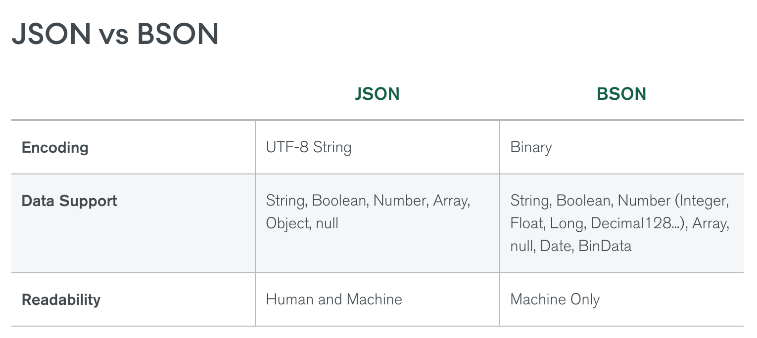
How BSON is stored in the MongoDB Database
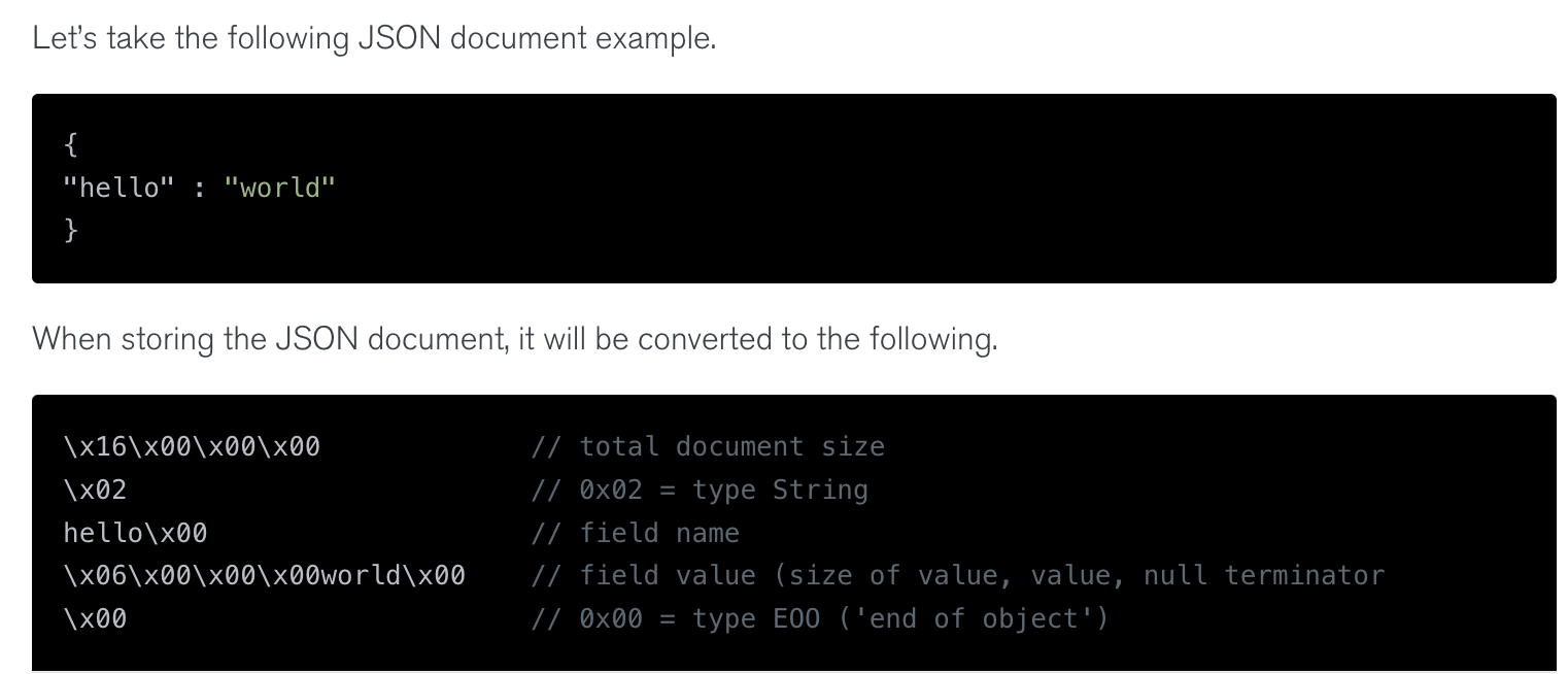
insertMany() is used to insert more than one document.
db.friendsCollection.insertMany([
{
"firstname": "Phoebe",
"lastname":"Buffay",
"age": 31,
"profession":"Therapist"
},
{
"firstname": "Ross",
"lastname":"Geller",
"age": 31,
"location": "NY",
"profession":"Palentologist",
"spouses":["Carol","Emily","Rachel"]
},
{
"firstname": "Chandler",
"lastname":"Bing",
"age": 31,
"location": "NY"
},
{
"firstname": "Joey",
"lastname":" Tribianni",
"age": 32,
"location": "NYC",
"profession":"actor"
}
])
db.friendsCollection.insertMany([
{
"firstname": "rachel",
"lastname" : "green",
"age" : 30,
"location": "NYC",
"profession":"Fashion Designer"
},
{
"name":{"firstname":"Ben",
"lastname" : "Geller"},
"age" : 6,
"location": "NYC"
},
{
"name":{"firstname":"Emma",
"lastname" : "Geller"},
"age" : 1,
"location": "NYC"
}
])
Index
MongoDB cannot create a unique index on the specified index field(s) if the collection already contains data that would violate the unique constraint for the index.
db.friendsCollection.createIndex({"firstname" : 1} , {unique : true})
[Avg. reading time: 2 minutes]
Querying MongoDB
2 ways to view the entire contents of collection
db.getCollection("friendsCollection").find()
db.friendsCollection.find()
Filter Documents
// exact match
db.friendsCollection.find(
{
age: 31
}
)
// less than
db.friendsCollection.find(
{
age : {$lt : 31}
}
)
// greater than
db.friendsCollection.find(
{
age : {$gt : 30}
}
)
// Between
db.friendsCollection.find(
{
age : {$gt : 29},
age : {$lt : 31}
}
)
// nested
db.friendsCollection.find({"name.firstname":"Ben"});
More Queries
Using Regular Expression
Regular expressions are used within two slashes / /
// Find firstnames containing letter R
db.friendsCollection.find({"firstname": /.*R.*/})
or
db.friendsCollection.find({"firstname": /R/})
// Find names starting with lower case r
db.friendsCollection.find({"firstname": /^r/})
// Find names ending with e
db.friendsCollection.find({"firstname": /e$/})
// case insensitive
db.friendsCollection.find({"firstname":{'$regex' : '^r', '$options' : 'i'}})
db.friendsCollection.find({"firstname":{"$regex" : "^r", "$options" : "i"}})
[Avg. reading time: 7 minutes]
Update & Remove
Update Statement
// Update Statement
db.friendsCollection.update({"firstname":"Ross"}, {$set: {age: 33}})
// Verify the update
db.friendsCollection.find({"firstname":{'$regex' : '^r', '$options' : 'i'}})
Remove Statement
// Remove the attribute / element
db.friendsCollection.update({"firstname": "Phoebe"}, {$unset: {age:""}});
// Remove entire document
db.friendsCollection.remove({firstname: "Ross"}, true);
db.friendsCollection.find();
// Remove all documents from friendsCollection
db.friendsCollection.remove({});
Drop Statement()
db.collection.drop()
Bulk Insert
Unordered Insert - Asynchronous
var bulk = db.students1.initializeUnorderedBulkOp();
bulk.insert( { firstname: "Sheldon", last_name: "Cooper" } );
bulk.insert( { firstname: "Jerry", last_name: "Seinfeld" } );
bulk.insert( { firstname: "Ray", last_name: "Ramona" } );
bulk.insert( { firstname: "Penny" } );
bulk.insert( { firstname: "Cosmo", last_name: "Kramer" } );
bulk.find({firstname:"Penny"}).update({$set:{lastname:"noName",gender:"F"}})
bulk.execute();
Asynchronous Execution: The operations can be executed in parallel or in any order, not necessarily the order in which they were added to the bulk operation. This can lead to performance benefits because MongoDB doesn't need to wait for one operation to complete before starting the next one.
Error Handling: If an error occurs, MongoDB will attempt to execute the rest of the operations in the bulk. It does not stop at the first error (unless the error is on the server side, like losing connection).
Use Case: Useful when the order of the operations does not affect the outcome and when performance is a priority over execution order.
Ordered Insert - Does in sequence
var bulk = db.students2.initializeOrderedBulkOp();
bulk.insert( { firstname: "Sheldon", last_name: "Cooper" } );
bulk.insert( { firstname: "Jerry", last_name: "Seinfeld" } );
bulk.insert( { firstname: "Ray", last_name: "Ramona" } );
bulk.insert( { firstname: "Penny" } );
bulk.insert( { firstname: "Cosmo", last_name: "Kramer" } );
bulk.find({firstname:"Penny"}).update({$set:{lastname:"noName",gender:"F"}})
bulk.execute();
Sequential Execution: The operations are executed in the exact order they were added to the bulk operation. If an operation fails, MongoDB stops processing any remaining operations in the bulk.
Error Handling: Stops at the first error encountered. This allows you to know exactly at which point the bulk operation failed, making debugging easier.
Use Case: Important when the order of operations affects the final state of the database. For example, if one operation depends on the result of a previous operation, ordered bulk operations ensure that these dependencies are respected.
[Avg. reading time: 1 minute]
Import
CSV to MongoDB
https://learn.mongodb.com/learn/course/importing-csv-data-into-mongodb/learning-byte/learn?_ga=2.95494940.102564042.1712084266-1489521210.1711814366
Download Books.json
https://www.mongodbtutorial.org/wp-content/uploads/2020/08/books.zip
mongoimport books.json -d bookdb -c books --drop
./mongoimport books.json --uri=mongodb+srv://..... t/ -d bookdb -c books --drop --mode=insert
[Avg. reading time: 1 minute]
Logical Operators
$and -- true when all the conditions are true, else false.
$or -- true when at-least one condition is true, else false.
$not -- negation true/false
$nor -- true when all conditions are false, false otherwise.
/ age > 31 and location = NYC
db.friendsCollection.find(
{
$and:
[
{age : {$gt : 31}}
,{location: "NYC"}
]
});
// Greater than or equal to 31 and name = Ross
db.friendsCollection.find(
{
$and:
[
{age : {$gte : 31}}
,{firstname: "Ross"}
]
});
[Avg. reading time: 10 minutes]
Data Types
- String: Refers to plain text
- Number: Consists of all numeric fields
- Boolean: Consists of True or False
- Object: Other embedded JSON objects
- Array: Collection of fields
- Null: Special value to denote fields without any value
{audience_rating: 6}
{audience_rating: 7.6}
{"title": "A Swedish Love Story", released: "1970-04-24"}
{"title": "A Swedish Love Story", released: "24-04-1970"}
{"title": "A Swedish Love Story", released: "24th April 1970"}
{"title": "A Swedish Love Story", released: "Fri, 24 Apr 1970"}
Variables
var name="Rachel Green"
name
var plainNum = 1299
plainNum
// forces MongoDB to use 32 bit
var explicitInt = NumberInt("1299")
explicitInt
// long forces 64 bit
var explicitLong = NumberLong("777888222116643")
explicitLong
var explicitLong_double = NumberLong(444333222111242)
explicitLong_double
// forces 128 bit
var explicitDecimal = NumberDecimal("142.42")
explicitDecimal
var explicitDecimal_double = NumberDecimal(142.42)
explicitDecimal_double
//values are rounded off
var decDbl = NumberDecimal(5999999999.99999999)
decDbl
// boolean demo
var isActive=true
isActive
var isDeleted=false
isDeleted
// objects
var friend={
"first_name":"Rachel",
"last_name":"Green",
"email":"rachel@friends.com"
}
friend
friend.first_name
<strong>var friends1=[
</strong>{
"firstname": "Phoebe",
"lastname":"Buffay",
"age": 31,
"profession":"Therapist"
},
{
"firstname": "Ross",
"lastname":"Geller",
"age": 31,
"location": "NY",
"profession":"Palentologist",
"spouses":["Carol","Emily","Rachel"]
},
{
"firstname": "Chandler",
"lastname":"Bing",
"age": 31,
"location": "NY"
},
{
"firstname": "Joey",
"lastname":" Tribianni",
"age": 32,
"location": "NYC",
"profession":"actor"
}
]
var friends2 = [
{
"firstname": "rachel",
"lastname" : "green",
"age" : 30,
"location": "NYC",
"profession":"Fashion Designer"
},
{
"name":{"firstname":"Ben",
"lastname" : "Geller"},
"age" : 6,
"location": "NYC"
},
{
"name":{"firstname":"Emma",
"lastname" : "Geller"},
"age" : 1,
"location": "NYC"
}
]
Skip - Limit
db.friendsCollection.find().sort({"lastname":1,"firstname":1}).limit(2)
db.friendsCollection.find().sort({"lastname":1,"firstname":1}).skip(2).limit(2)
Sort
db.friendsCollection.drop()
db.friendsCollection.insertMany(friends1)
db.friendsCollection.insertMany(friends2)
db.friendsCollection.find().sort({"firstname":1})
db.friendsCollection.find().sort({"firstname":-1})
Projection
MongoDB projections specify which fields should be returned in the documents that match a query. All fields are returned by default, but you can include or exclude specific fields to control the amount of data MongoDB returns.
Projections can help improve performance by reducing network bandwidth and processing time, especially for documents with large amounts of data or when you only need a subset.
Return firstname and lastname only
This query tells MongoDB to return only the firstname and profession fields of all documents in the friends1 collection. If you want to exclude the _id field as well, you can do so by explicitly setting it to 0 in the projection:
db.friendsCollection.find({},{"firstname":1,"lastname":1})
db.friendsCollection.find({},{"_id":0,"firstname":1,"lastname":1})
// Exclude Location
db.friendsCollection.find({ firstname: "Joey" }, { location: 0 })
db.friendsCollection.find({}, { "name.firstname": 1, age: 1 })
Distinct Count
db.friendsCollection.distinct("lastname")
db.friendsCollection.distinct("lastname",{"email":{$regex:".*friends"}})
db.friendsCollection.count()
// without condition, this will check the metadata and return the count.
// It will not be accurate all the time due to multi-node architecture
// and the time taken to sync.
db.friendsCollection.count({"lastname":"Geller"})
// newer syntaxes always query need to be passed, it’s slower
db.friendsCollection.countDocuments({"lastname":"Geller"})
// newer syntaxes to get an overall idea using metadata, quick result
db.friendsCollection.estimatedDocumentCount({"lastname":"Geller"})
Array Slice
db.friendsCollection.find({"firstname":{$eq:"Ross"}}, {"spouses":{$slice:1}})
db.friendsCollection.find({"firstname":{$eq:"Ross"}}, {"spouses":{$slice:-1}})
[Avg. reading time: 1 minute]
Operators
Comparison Operators
| MySQL | MongoDB |
|---|---|
| = | $eq |
| <> | $ne |
| > | $gt |
| < | $lt |
| >= | $gte |
| <= | $lte |
| in | $in |
| not in | $nin |
Example
//
db.friendsCollection.find(
{"lastname":{$nin:["Geller","Green"]}}
)
//
db.friendsCollection.find(
{"lastname":{$nin:["Geller","Green"]}}
).count()
Logical Operators
| MySQL | MongoDB |
|---|---|
| and | $and |
| or | $or |
| not | $not |
[Avg. reading time: 9 minutes]
Aggregation Pipeline
MongoDB is not just adding and filtering data using find()
Aggregation is a way of processing a large number of documents in a collection by means of passing them through different stages.
The stages make up what is known as a pipeline. The stages in a pipeline can filter, sort, group, reshape and modify documents that pass through the pipeline
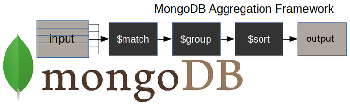
$matchstage – filters those documents we need to work with, those that fit our needs$groupstage – does the aggregation job$sortstage – sorts the resulting documents the way we require (ascending or descending)
use sampleagg;
db.states.insertMany(
[
{ "_id": "NY", "name": "New York", "population": 19453561, "rank": 4 },
{ "_id": "CA", "name": "California", "population": 39512223, "rank": 1 },
{ "_id": "TX", "name": "Texas", "population": 28995881, "rank": 2 },
{ "_id": "NJ", "name": "New Jersey", "population": 8995881, "rank": 3 }
]
)
db.universities.insertMany(
[
{ "name": "Columbia University", "stateId": "NY", "year": 2020, "enrolled": 31000, "graduated": 7000 },
{ "name": "New York University", "stateId": "NY", "year": 2020, "enrolled": 51123, "graduated": 12000 },
{ "name": "University of California, Berkeley", "stateId": "CA", "year": 2020, "enrolled": 43000, "graduated": 10000 },
{ "name": "Stanford University", "stateId": "CA", "year": 2020, "enrolled": 17400, "graduated": 4000 },
{ "name": "University of Texas at Austin", "stateId": "TX", "year": 2020, "enrolled": 51000, "graduated": 11000 },
{ "name": "Rowan University", "stateId": "NJ", "year": 2020, "enrolled": 19500, "graduated": 4300 },
{ "name": "Rutgers University", "stateId": "NJ", "year": 2020, "enrolled": 70645, "graduated": 17600 }
]
)
db.universities.find()
// Step 1
db.universities.aggregate([
{
$match: {
"year": 2020 // Focus on the year 2020
}
},
{
$project: {
_id:1,
name:1,
stateId:1,
year:1,
enrolled:1,
graduated:1
}
}
])
// Step 2
// Group by State, and do a sum of Enrolled, Graduated
// In MongoDB count is not part of Grouping.
db.universities.aggregate([
{
$match: {
"year": 2020 // Focus on the year 2020
}
},
{
$group: {
_id: "$stateId", // Group by state ID
totalEnrolled: { $sum: "$enrolled" }, // Sum of all students enrolled
totalGraduated: { $sum: "$graduated" }, // Sum of all graduates
universitiesCount: { $sum: 1 } // Count universities
}
},
{
$project: {
_id:1,
totalEnrolled:1,
totalGraduated:1,
universitiesCount:1
}
}
])
// Step 3
// Join with State Documents
db.universities.aggregate([
{
$match: {
"year": 2020 // Focus on the year 2020
}
},
{
$group: {
_id: "$stateId", // Group by state ID
totalEnrolled: { $sum: "$enrolled" }, // Sum of all students enrolled
totalGraduated: { $sum: "$graduated" }, // Sum of all graduates
universitiesCount: { $sum: 1 } // Count universities
}
},
{
$lookup:{
from:"states",
localField:"_id",
foreignField: "_id",
as:"stateDetails"
}
},
{
$project: {
_id:1,
totalEnrolled:1,
totalGraduated:1,
universitiesCount:1,
stateDetails:1
}
}
])
// Step 4
// Final Query
// is used to deconstruct the stateDetails array resulting from the $lookup,
// making it easier to work with the state details in subsequent stages.
db.universities.aggregate([
{
$match: {
"year": 2020 // Focus on the year 2020
}
},
{
$group: {
_id: "$stateId", // Group by state ID
totalEnrolled: { $sum: "$enrolled" }, // Sum of all students enrolled
totalGraduated: { $sum: "$graduated" }, // Sum of all graduates
universitiesCount: { $sum: 1 } // Count universities
}
},
{
$lookup:{
from:"states",
localField:"_id",
foreignField: "_id",
as:"stateDetails"
}
},
{
$unwind: "$stateDetails"
},
{
$project: {
_id: 1,
totalEnrolled:1,
totalGraduated:1,
universitiesCount:1,
"stateName": "$stateDetails.name",
"statePopulation": "$stateDetails.population",
"stateRank": "$stateDetails.rank",
}
}
])
[Avg. reading time: 1 minute]
Further Reading
MongoDB Certification Program
For students they offer Free Certification Opportunity
[Avg. reading time: 1 minute]
Fun Task
How will you Model a Tweet into a JSON Document. Remember it's not just creating Key: Value pairs.
(This is to test your design not how Twitter does it)
creation date and time
user name
actual name
user profile pic
user verification status (paid or celebrity or company)
hash tags
mentions
tweet text
likes
comments
retweets
tweet status
bookmarks
[Avg. reading time: 1 minute]
Sample
{
"tweet": {
"tweet_text": "Exploring the world of MongoDB. #NOSQL #MongoDB",
"creation_date_time": "2021-04-02T12:34:56Z",
"likes": 300,
"comments": 45,
"retweets": 150,
"bookmarks": 75,
"tweet_status": "active",
"hashtags": [
{
"tag": "NOSQL"
},
{
"tag": "MongoDB"
}
],
"mentions": [
{
"screen_name": "mongodb",
"user_id": "1122334455"
}
]
},
"user": {
"user_name": "sql_guru",
"actual_name": "db Enthusiast",
"profile_pic": "https://example.com/profile_pic.jpg",
"verification_status": {
"type": "celebrity",
"verified": true
}
}
}
[Avg. reading time: 1 minute]
Linux Fundamentals
[Avg. reading time: 1 minute]
Overview
Windows
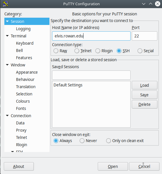
enter your_rowan_id (not email / not banner)
enter password (it won’t display *)
Mac / Linux
Terminal
$ ssh your_rowan_id@elvis.rowan.edu (not email / not banner)
enter password (it won’t display *)
[Avg. reading time: 2 minutes]
CSVSQL
SQL query on CSV file
Simple query
csvsql --query "select * from sales_100" ./sales_100.csv
with Limit
csvsql --query "select * from sales_100 limit 5" ./sales_100.csv
using MAX aggregate function
csvsql --query "select max(unitprice) from sales_100 limit 5" ./sales_100.csv
Use double quotes to handle columns that have Space in between them in csvsql
csvsql --query 'select distinct("Order Priority") from sales_100' ./sales_100.csv
Using Group By
csvsql --query "select country,region,count(*) from sales_100 group by country, region" ./sales_100.csv
using WildCards
csvsql --query "select * from sales_100 where region like 'A%' order by region desc" sales_100.csv
````<span id='footer-class'>Ver 5.5.9</span>
<footer id="last-change">Last change: 2025-12-03</footer>````[Avg. reading time: 1 minute]
Linux Commands - 01
The first set of Linux commands users should be familiar with are
hostname
whoami
uname
uname -a
ping
pwd
echo ""
mkdir <foldername>
cd <foldername>
touch <filename>
echo "sometext" > <filename>
cd .. (space is needed)
ls [-l]
cp <filename> <filename1>
````<span id='footer-class'>Ver 5.5.9</span>
<footer id="last-change">Last change: 2025-12-03</footer>````[Avg. reading time: 0 minutes]
Linux Commands - 02
wget
touch
echo
variables
|
cat
wc
more
head
tail
grep
cut
uniq
sort
````<span id='footer-class'>Ver 5.5.9</span>
<footer id="last-change">Last change: 2025-12-03</footer>````[Avg. reading time: 5 minutes]
AWK
AWK is a scripting language used for manipulating data and generating reports. It’s a Domain Specific Language.
Demo Using AWK
wget
https://raw.githubusercontent.com/gchandra10/awk_scripts_data_science/master/sales_100.csv
Display file contents
awk '{print }' sales_100.csv
By default, AWK uses space as a delimiter. Since our file has a comma (,) let’s specify it with -F
awk -F ',' '{print }' sales_100.csv
To get the number of columns of each row, use the NF (a predefined variable)
awk -F ',' '{print NF}' sales_100.csv
AWK lets you choose specific columns.
awk -F ',' '{print $1,$2,$4}' sales_100.csv
Row Filter
AND = &&
OR = ||
Not = !
awk -F ',' '{if($4 == "Online") {print $1,$2,$4}}' sales_100.csv
awk -F ',' '{if($4 == "Online" && $5 =="L") {print $1,$2,$4,$5}}' sales_100.csv```
Variables
awk -F ',' '{sp=$9 * $10;cp=$9 * $11; {printf "%f,%f,%s,%s \n",sp,cp,$1,$2 }}' sales_100.csv
RegEx: Return all rows starting with A in Column 1
awk -F ',' '$1 ~ /^A/ {print}' sales_100.csv
Return all rows which have Space in Column 1
awk -F ',' '$1 ~ /\s/ {print}' sales_100.csv
AWK also has the functionality to change the column and row delimiter
OFS: Output Field Separator
ORS: Output Row Separator
awk -F ',' 'BEGIN{OFS="|";ORS="\n\n"} $1 ~ /^A/ {print substr($1,1,4),$2,$3,$4,$5}' sales_100.csv
Built-in Functions
awk -F ',' 'BEGIN{OFS="|";ORS="\n"} $1 ~ /^A/ {print tolower(substr($1,1,4)),tolower($2),$3,$4,$5}' sales_100.csv
````<span id='footer-class'>Ver 5.5.9</span>
<footer id="last-change">Last change: 2025-12-03</footer>````[Avg. reading time: 2 minutes]
CSVGREP
-c column -m filter
csvgrep -c Region -m Europe sales_100.csv
Using Regular expression to find Regions starting with A
csvgrep -c Region -r ^A. sales_100.csv
Combining Grep, Cut, and Look
csvgrep -c Region -m Europe sales_100.csv | csvcut -c 1,2 | csvlook
Inverse Matching
csvgrep -i -c Region -n region -m Europe sales_100.csv | csvlook
Sorting data
Sorting on Region column
csvsort -c Region sales_100.csv | csvlook --max-rows 3
Sorting in Reverse Order on Region Column
csvsort -r -c Region sales_100.csv | csvlook --max-rows 3
[Avg. reading time: 3 minutes]
CSVKIT
Install csvkit (windows / Linux / mac)
pip install csvkit
To get a list of Column Names from CSV
csvcut -n sales_100.csv
Quick stats about the CSV file such as number of columns, sample values, does it contain NULL or not
csvstat sales_100.csv
View the CSV in Table format
csvlook sales_100.csv
csvlook --max-rows 2 sales_100.csv
csvlook -l --max-rows 20 sales_100.csv
To view selected columns, use csvcut.
csvcut -c 1,2,4 sales_100.csv
csvcut -c 1,2,4 sales_100.csv | csvlook
To see the result with Line Numbers, use param -l
csvcut -c 1,2,4 sales_100.csv | csvlook -l
Instead of column numbers, column names can also be used
csvcut -c Region,Country sales_100.csv | csvlook -l
Exclude selected columns
csvcut -C Region,Country sales_100.csv | csvlook
Change column delimiter
csvformat -D "|" sales_100.csv
[Avg. reading time: 1 minute]
Tools
[Avg. reading time: 3 minutes]
CICD Intro
A CI/CD Pipeline is simply a development practice. It tries to answer this one question: How can we ship quality features to our production environment faster?
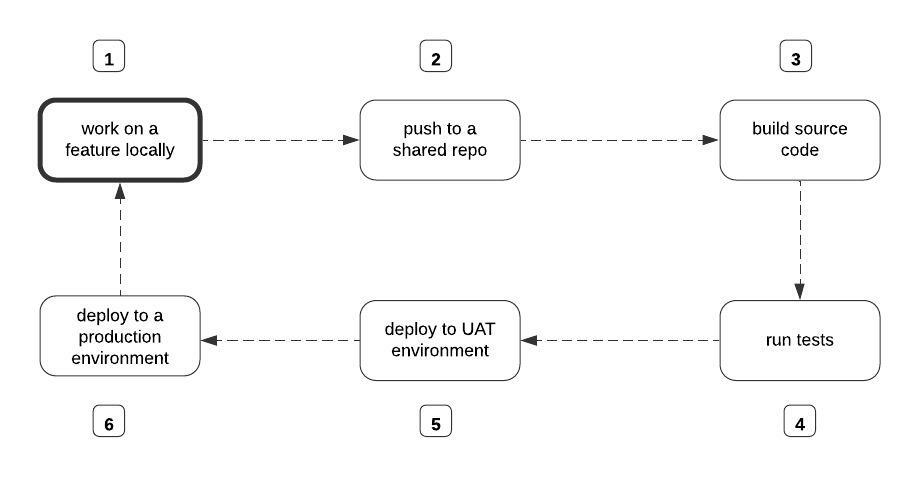 src: https://www.freecodecamp.org/
Without the CI/CD Pipeline, the developer will manually perform each step in the diagram above. To build the source code, someone on your team has to run the command to initiate the build process manually.
Continuous Integration (CI)
Automatically tests code changes in a shared repository. Ensures that new code changes don’t break the existing code.
Continuous Delivery (CD)
Automatically deploys all code changes to a testing or staging environment after the build stage, then manually deploys them to production.
Continuous Deployment
This happens when an update in the UAT environment is automatically deployed to the production environment as an official release.
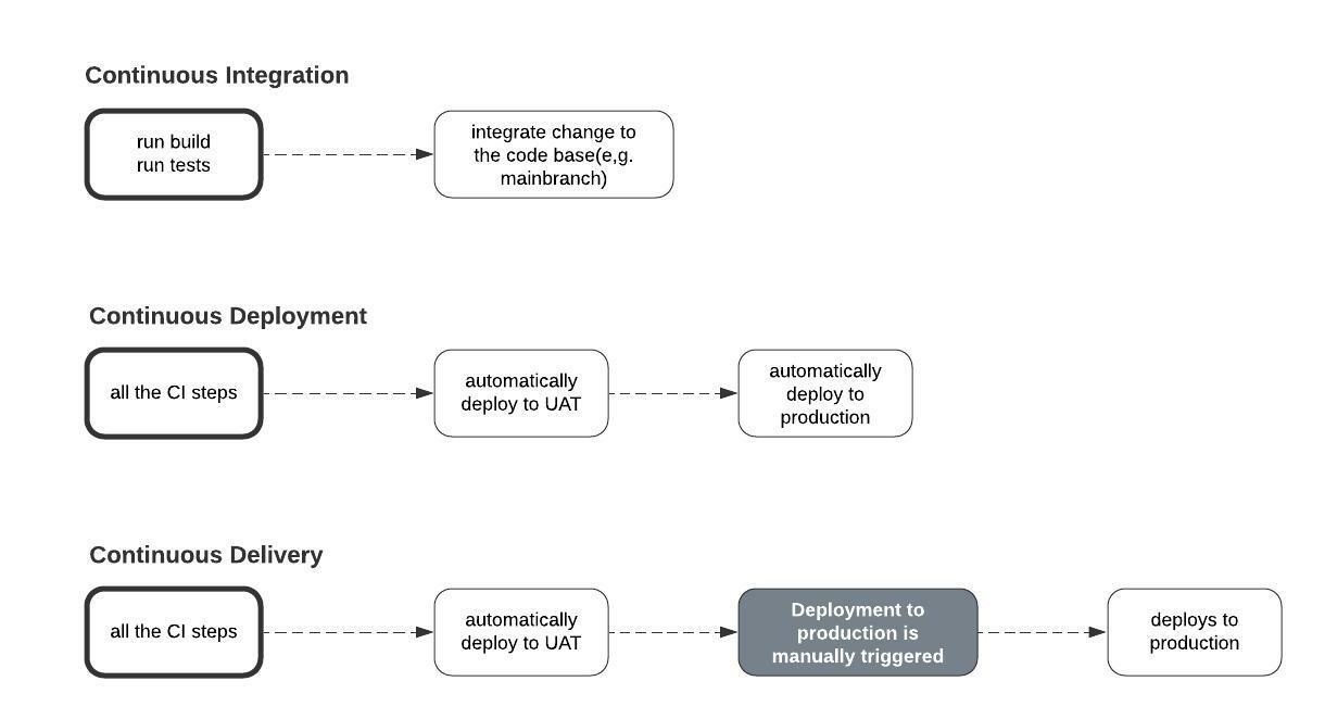
src: https://www.freecodecamp.org/
[Avg. reading time: 6 minutes]
CICD Tools
On-Prem & Web
- Jenkins
- Circle CI
Web Based
- GitHub Actions
- GitLab
Cloud Providers
- AWS CodeBuild
- Azure DevOps
- Google Cloud Build
GitHub Actions
Free and Popular
Five Concepts
Workflows
Automated processes that contain one or more logical jobs. Entire to-do list.
Jobs
Tasks you command GitHub Action to execute. It consists of steps that GitHub Actions will execute on a runner.
Events
Trigger the execution of the job.
- on push / pull
- on schedule
- on workflow_dispatch (Manual Trigger)
Actions
Reusable commands that can be used in your config file.
https://github.com/features/actions
Runners
Remote computer that GitHub Actions uses to execute the jobs.
Github-Hosted Runners
- ubuntu-latest
- windows-latest
- macos-latest
Self-Hosted Runners
- Specific OS that Github does not offer.
- Connection to a private network/environment.
- To save costs for projects with high usage. (Enterprise plans are expensive)
YAML (Yet Another Markup Language)
YAML is a human-friendly data serialization
language for all programming languages.
https://learnxinyminutes.com/docs/yaml/
Sample
name: Multi-Event Workflow
on:
push:
branches: [main]
pull_request:
branches: [main]
workflow_dispatch:
inputs:
manualParam:
description: 'Input for manual triggers'
required: false
default: 'Default value'
schedule:
- cron: '0 0 * * *' # Runs at 00:00 UTC every day
jobs:
build-and-test:
runs-on: ubuntu-latest
steps:
- uses: actions/checkout@v2
- name: Set up Python
uses: actions/setup-python@v2
with:
python-version: '3.8'
- name: Install dependencies
run: |
python -m pip install --upgrade pip
pip install -r requirements.txt
- name: Run tests
run: |
echo "Run your tests or scripts here."
echo "Manual trigger parameter value: ${{ github.event.inputs.manualParam }}"
DEMO
Multiple Runners Demo
https://github.com/gchandra10/github-actions-multiple-runners-demo
https://github.com/gchandra10/python_cicd_calculator
[Avg. reading time: 3 minutes]
CI YAML
name: Build and Test
on:
push:
branches: [ main ]
pull_request:
branches: [ main ]
jobs:
test:
runs-on: ubuntu-latest
steps:
- name: Checkout code
uses: actions/checkout@v2
- name: Set up Python Environment
uses: actions/setup-python@v2
with:
python-version: '3.x'
- name: Install Dependencies
run: |
python -m pip install --upgrade pip
pip install -r requirements.txt
- name: Run Tests
run: |
python -m unittest test_calc.py -v
- name: Send Discord Failure Notification
# https://github.com/marketplace/actions/actions-for-discord
if: failure()
env:
DISCORD_WEBHOOK: ${{ secrets.DISCORD_WEBHOOK }}
uses: Ilshidur/action-discord@master
with:
args: '@here :x: The Calculator App integration {{ EVENT_PAYLOAD.repository.full_name }} test failed. Check the Run id ${{ github.run_id }} on Github for details.'
- name: Send Discord Success Notification
# https://github.com/marketplace/actions/actions-for-discord
if: success()
env:
DISCORD_WEBHOOK: ${{ secrets.DISCORD_WEBHOOK }}
uses: Ilshidur/action-discord@master
with:
args: ' :white_check_mark: The Calculator App {{ EVENT_PAYLOAD.repository.full_name }} - ${{ github.run_id }} successfully integrated and tested.'
[Avg. reading time: 2 minutes]
CD Yaml
- name: Deploy to Server
if: success()
uses: appleboy/ssh-action@master
with:
host: ${{ secrets.SERVER_HOST }}
username: ${{ secrets.SERVER_USER }}
key: ${{ secrets.SSH_PRIVATE_KEY }}
port: 22 # Optional if your SSH server uses a different port
script: |
cd /path/to/your/project
git pull
# Any other deployment or restart service commands
- name: Configure AWS Credentials
uses: aws-actions/configure-aws-credentials@v1
with:
aws-access-key-id: ${{ secrets.AWS_ACCESS_KEY_ID }}
aws-secret-access-key: ${{ secrets.AWS_SECRET_ACCESS_KEY }}
aws-region: your-aws-region
- name: Deploy to AWS Lambda
run: |
# Package your application
zip -r package.zip .
# Deploy/update your Lambda function
aws lambda update-function-code --function-name your-lambda-function-name --zip-file fileb://package.zip
[Avg. reading time: 6 minutes]
Containers
World before containers
Physical Machines
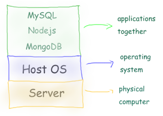
- 1 Physical Server
- 1 Host Machine (say some Linux)
- 3 Applications installed
Limitation:
- Need of physical server.
- Version dependency (Host and related apps)
- Patches ”hopefully” not affecting applications.
- All apps should work with the same Host OS.
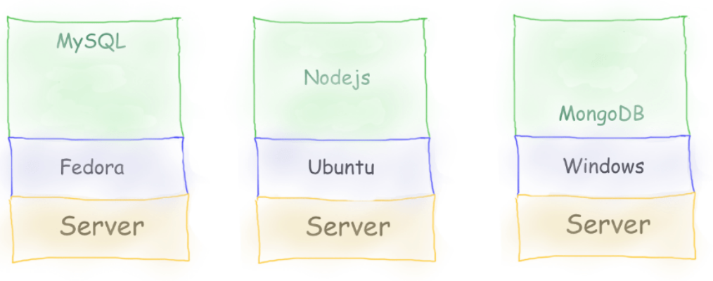
- 3 physical server
- 3 Host Machine (diff OS)
- 3 Applications installed
Limitation:
- Need of physical server(s).
- Version dependency (Host and related apps)
- Patches ”hopefully” not affecting applications.
- Maintenance of 3 machines.
- Network all three so they work together.
Virtual Machines
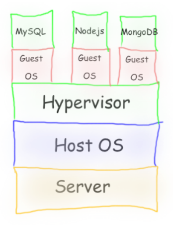
-
Virtual Machines emulate a real computer by virtualizing it to execute applications,running on top of a real computer.
-
To emulate a real computer, virtual machines use a Hypervisor to create a virtual computer.
-
On top of the Hypervisor, we have a Guest OS that is a Virtualized Operating System where we can run isolated applications, called Guest Operating System.
-
Applications that run in Virtual Machines have access to Binaries and Libraries on top of the operating system.
( + ) Full Isolation, Full virtualization ( - ) Too many layers, Heavy-duty servers.
Here comes Containers
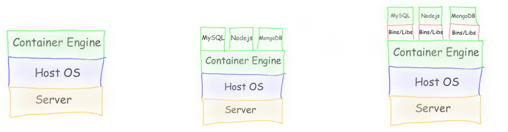
Containers are lightweight, portable environments that package an application with everything it needs to run—like code, runtime, libraries, and system tools—ensuring consistency across different environments. They run on the same operating system kernel and isolate applications from each other, which improves security and makes deployments easier.
-
Containers are isolated processes that share resources with their host and, unlike VMs, don’t virtualize the hardware and don’t need a Guest OS.
-
Containers share resources with other Containers in the same host.
-
This gives more performance than VMs (no separate guest OS).
-
Container Engine in place of Hypervisor.
Pros
- Isolated Process
- Mounted Files
- Lightweight Process
Cons
- Same Host OS
- Security
[Avg. reading time: 9 minutes]
VMs or Containers
VMs are great for running multiple, isolated OS environments on a single hardware platform. They offer strong security isolation and are useful when applications need different OS versions or configurations.
Containers are lightweight and share the host OS kernel, making them faster to start and less resource-intensive. They’re perfect for microservices, CI/CD pipelines, and scalable applications.
Smart engineers focus on the right tool for the job rather than getting caught up in “better or worse” debates.
Use them in combination to make life better.
Popular container technologies
Docker: The most widely used container platform, known for its simplicity, portability, and extensive ecosystem.
Podman: A daemonless container engine that’s compatible with Docker but emphasizes security, running containers as non-root users.
Podman stands out because it aligns well with Kubernetes, which uses pods (groups of one or more containers) as the basic building block. Podman operates directly with pods without needing a daemon, making running containers without root privileges simpler and safer.
This design reduces the risk of privilege escalation attacks, making it a preferred choice in security-sensitive environments. Plus, Podman can run existing Docker containers without modification, making it easy to switch over.
NOTE: INSTALL DOCKER OR PODMAN (Not BOTH)
Podman on Windows
https://podman-desktop.io/docs/installation/windows-install
Once installed, verify the installation by checking the version:
podman info
Podman on MAC
After installing, you need to create and start your first Podman machine:
podman machine init
podman machine start
You can then verify the installation information using:
podman info
Podman on Linux
You can then verify the installation information using:
podman info
Docker Installation
Here is step by step installation
https://docs.docker.com/desktop/setup/install/windows-install/
[Avg. reading time: 1 minute]
What container does
It brings to us the ability to create applications without worrying about their environment.

[Avg. reading time: 2 minutes]
Containers
Images
The image is the prototype or skeleton to create a container, like a recipe to make your favorite food.
Container
A container is the environment, up and running and ready for your application.
If Image = Recipe, then Container = Cooked food.
Where to get the Image from?
Docker Hub
For both Podman and Docker, images are from the Docker Hub.
[Avg. reading time: 13 minutes]
Container Examples
If you have installed Docker replace podman with docker.
Syntax
podman pull <imagename>
podman run <imagename>
OR
docker pull <imagename>
docker run <imagename>
Examples:
podman pull hello-world
podman run hello-world
podman container ls
podman container ls -a
podman image ls
docker pull hello-world
docker run hello-world
docker container ls
docker container ls -a
docker image ls
Optional Setting (For PODMAN)
/etc/containers/registries.conf
unqualified-search-registries = ["docker.io"]
Deploy MySQL Database using Containers
Create the following folder
Linux / Mac
mkdir -p container/mysql
cd container/mysql
Windows
md container
cd container
md mysql
cd mysql
Note: If you already have MySQL Server installed in your machine then please change the port to 3307 as given below.
-p 3307:3306 \
Run the container
podman run --name mysql -d \
-p 3306:3306 \
-e MYSQL_ROOT_PASSWORD=root-pwd \
-e MYSQL_ROOT_HOST="%" \
-e MYSQL_DATABASE=mydb \
-e MYSQL_USER=remote_user \
-e MYSQL_PASSWORD=remote_user-pwd \
docker.io/library/mysql:8.4.4
OR
docker run --name mysql -d \
-p 3306:3306 \
-e MYSQL_ROOT_PASSWORD=root-pwd \
-e MYSQL_ROOT_HOST="%" \
-e MYSQL_DATABASE=mydb \
-e MYSQL_USER=remote_user \
-e MYSQL_PASSWORD=remote_user-pwd \
docker.io/library/mysql:8.4.4
-d : detached (background mode)
-p : 3306:3306 maps mysql default port 3306 to host machines port 3306
3307:3306 maps mysql default port 3306 to host machines port 3307
-e MYSQL_ROOT_HOST="%" Allows to login to MySQL using MySQL Workbench
Login to MySQL Container
podman exec -it mysql bash
List all the Containers
podman container ls -a
or
docker container ls -a
Stop MySQL Container
podman stop mysql
or
docker stop mysql
Delete the container**
podman rm mysql
or
docker rm mysql
Preserve the Data for future**
Inside container/mysql
mkdir data
podman run --name mysql -d \
-p 3306:3306 \
-e MYSQL_ROOT_PASSWORD=root-pwd \
-e MYSQL_ROOT_HOST="%" \
-e MYSQL_DATABASE=mydb \
-e MYSQL_USER=remote_user \
-e MYSQL_PASSWORD=remote_user-pwd \
-v ./data:/var/lib/mysql \
docker.io/library/mysql:8.4.4
or
docker run --name mysql -d \
-p 3306:3306 \
-e MYSQL_ROOT_PASSWORD=root-pwd \
-e MYSQL_ROOT_HOST="%" \
-e MYSQL_DATABASE=mydb \
-e MYSQL_USER=remote_user \
-e MYSQL_PASSWORD=remote_user-pwd \
-v ./data:/var/lib/mysql \
docker.io/library/mysql:8.4.4
-- Create database
CREATE DATABASE IF NOT EXISTS friends_tv_show;
USE friends_tv_show;
-- Create Characters table
CREATE TABLE characters (
character_id INT AUTO_INCREMENT PRIMARY KEY,
first_name VARCHAR(50) NOT NULL,
last_name VARCHAR(50) NOT NULL,
actor_name VARCHAR(100) NOT NULL,
date_of_birth DATE,
occupation VARCHAR(100),
apartment_number VARCHAR(10)
);
INSERT INTO characters (first_name, last_name, actor_name, date_of_birth, occupation, apartment_number) VALUES
('Ross', 'Geller', 'David Schwimmer', '1967-10-02', 'Paleontologist', '3B'),
('Rachel', 'Green', 'Jennifer Aniston', '1969-02-11', 'Fashion Executive', '20'),
('Chandler', 'Bing', 'Matthew Perry', '1969-08-19', 'IT Procurement Manager', '19'),
('Monica', 'Geller', 'Courteney Cox', '1964-06-15', 'Chef', '20'),
('Joey', 'Tribbiani', 'Matt LeBlanc', '1967-07-25', 'Actor', '19'),
('Phoebe', 'Buffay', 'Lisa Kudrow', '1963-07-30', 'Massage Therapist/Musician', NULL);
select * from characters;
Build your own Image
mkdir -p container
cd container
Python Example
Follow the README.md
Fork & Clone
git clone https://github.com/gchandra10/docker_mycalc_demo.git
Web App Demo
Fork & Clone
git clone https://github.com/gchandra10/docker_webapp_demo.git
Publish Image to Docker Hub
Login to Docker Hub
- Create a Repository “my_faker_calc”
- Under Account Settings
- Personal Access Token
- Create a PAT token with Read/Write access for 1 day
Replace gchandra10 with yours.
podman login docker.io
or
docker login
enter userid
enter PAT token
Then build the Image with your userid
podman build -t gchandra10/my_faker_calc:1.0 .
podman image ls
or
docker build -t gchandra10/my_faker_calc:1.0 .
docker image ls
Copy the ImageID of gchandra10/my_fake_calc:1.0
Tag the ImageID with necessary version and latest
podman image tag <image_id> gchandra10/my_faker_calc:latest
or
docker image tag <image_id> gchandra10/my_faker_calc:latest
Push the Images to Docker Hub (version and latest)
podman push gchandra10/my_faker_calc:1.0
podman push gchandra10/my_faker_calc:latest
or
docker push gchandra10/my_faker_calc:1.0
docker push gchandra10/my_faker_calc:latest
Image Security
Open Source tool Trivy
https://trivy.dev/latest/getting-started/installation/
trivy image python:3.9-slim
trivy image gchandra10/my_faker_calc
trivy image gchandra10/my_faker_calc --severity CRITICAL,HIGH --format table
trivy image gchandra10/my_faker_calc --severity CRITICAL,HIGH --output result.txt
#podman #docker #container #dockerhub
[Avg. reading time: 6 minutes]
Overview
Definitions
Hardware: physical computer / equipment / devices
Software: programs such as operating systems, Word, Excel
Web Site: Readonly web pages such as company pages, portfolios, newspapers
Web Application: Read Write - Online forms, Google Docs, email, Google apps
Cloud Plays a significant role in the Big Data world.
In today’s market, Cloud helps companies to accommodate the ever-increasing volume, variety, and velocity of data.
Cloud Computing is a demand delivery of IT resources over the Internet through Pay Per Use.

src: https://thinkingispower.com/the-blind-men-and-the-elephant-is-perception-reality/
Without Cloud knowledge, knowing Bigdata will be something like the above picture.
- Volume: Size of the data.
- Velocity: Speed at which new data is generated.
- Variety: Different types of data.
- Veracity: Trustworthiness of the data.
- Value: Usefulness of the data.
- Vulnerability: Security and privacy aspects.
When people focus on only one aspect without the help of cloud technologies, they miss out on the comprehensive picture. Cloud solutions offer ways to manage all these dimensions in an integrated manner, thus providing a fuller understanding and utilization of Big Data.
Advantages of Cloud Computing for Big Data
- Cost Savings
- Security
- Flexibility
- Mobility
- Insight
- Increased Collaboration
- Quality Control
- Disaster Recovery
- Loss Prevention
- Automatic Software Updates
- Competitive Edge
- Sustainability
Types of Cloud Computing
Public Cloud
Owned and operated by third-party providers. (AWS, Azure, GCP, Heroku, and a few more)
Private Cloud
Cloud computing resources are used exclusively by a single business or organization.
Hybrid
Public + Private: By allowing data and applications to move between private and public clouds, a hybrid cloud gives your business greater flexibility, and more deployment options, and helps optimize your existing infrastructure, security, and compliance.
[Avg. reading time: 19 minutes]
Types of Cloud Services
SaaS - Software as a Service
Cloud-based service providers offer end-user applications. Google Apps, DropBox, Slack, etc.
Key Characteristics:
-
Web Access to Software: Users access the software via the internet, typically through a web browser.
-
Central Management: Software is managed from a central location by the service provider.
-
Multi-Tenant Model: One version of the application is used by multiple customers. Automatic Updates: No need for manual patches or upgrades; updates are handled by the provider.
When Not to Use SaaS:
-
Limited Internet Access
-
Mission-Critical Applications with Low Tolerance for Downtime
-
Highly Customized Applications: Business requires deep customization that SaaS platforms can’t accommodate
-
Hardware Integration Needs: When integration with on-premise hardware (e.g., scanners, local printers) is required.
-
Performance Demands: When very high performance or faster processing is critical and might be constrained by the internet connection.
-
Data Residency Requirements: When data must remain on-premise due to legal, security, or compliance reasons.
PaaS - Platform as a Service
PaaS provides a platform allowing customers to develop, run, and manage applications without dealing with the underlying infrastructure. Examples include AWS RDS, Heroku, and Salesforce.
Key Characteristics:
-
Scalable: Automatically scales resources up or down based on demand.
-
Built on Virtualization Technology: Uses virtual machines or containers to deliver resources.
-
Managed Services: Providers handle software updates, patches, and maintenance tasks, freeing up user resources to focus on development.
When Not to Use PaaS:
-
Vendor Lock-In: Proprietary tools or services (e.g., AWS-specific services) can limit portability, making it difficult to switch providers without significant rework.
-
Limited Control Over Infrastructure: When you need deep control over the underlying hardware, operating system, or network configurations, which PaaS typically abstracts away.
-
Specific Compliance Requirements: When the application has specific regulatory or compliance needs that PaaS providers cannot meet, such as data sovereignty or special security measures.
-
Incompatible with New or Niche Software: When using new or niche software that is not supported by the PaaS environment, requiring custom installations or configurations that PaaS platforms do not permit.
-
Performance-Sensitive Applications: When extremely high performance or low-latency connections are necessary, and PaaS may introduce limitations or overhead that impact performance.
-
Custom Middleware or Legacy Systems Integration: When applications require specific middleware or have dependencies on legacy systems that are not easily integrated with PaaS offerings.
IaaS - Infrastructure as a Service
IaaS provides virtualized computing resources over the internet, including servers, storage, and networking on a pay-as-you-go basis. Examples include Amazon EC2, Google Compute Engine, and S3.
Key Characteristics:
-
Highly Flexible and Scalable: Allows users to scale resources up or down based on needs, providing a high degree of control over the infrastructure.
-
Multi-User Access: Multiple users can access and manage the resources, facilitating collaboration and resource sharing.
-
Cost-Effective: Can be cost-effective when resources are used and managed efficiently, with the ability to pay only for what you use.
When Not to Use IaaS:
-
Complexity in Management: Requires managing and configuring virtual machines, networks, and storage, which can be complex and time-consuming compared to PaaS or SaaS.
-
Inexperienced Teams: When the team lacks expertise in managing infrastructure, leading to potential security risks, misconfigurations, or inefficient use of resources.
-
Maintenance Overhead: Users are responsible for managing OS updates, security patches, and application installations, which can increase the operational burden.
-
Predictable Workloads: For workloads that are highly predictable and stable, other models (like PaaS or even traditional on-premises solutions) might offer more streamlined management.
-
High Availability and Disaster Recovery: Setting up high availability, redundancy, and disaster recovery in IaaS requires careful planning and additional configuration, which can add complexity and cost.
-
Compliance and Security: If the application has stringent compliance and security needs, the responsibility lies with the user to ensure the infrastructure meets these requirements, which can be resource-intensive.
Comparison between Services
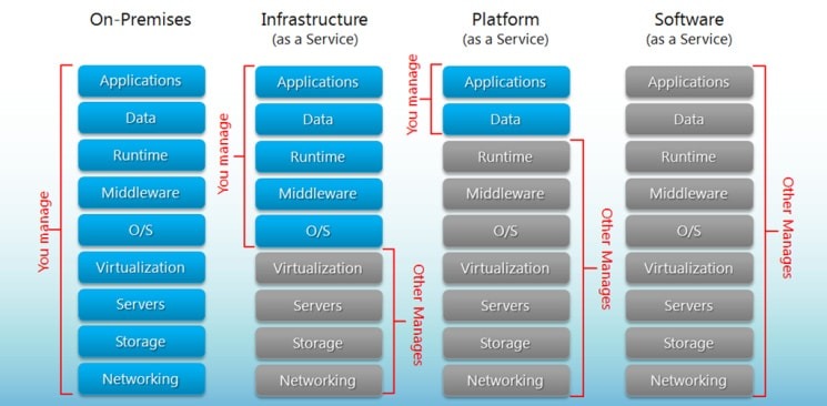
FaaS - Function as a Service (Serverless computing)
FaaS allows developers to run small pieces of code (functions) in response to events without managing the underlying infrastructure. This enables a serverless architecture where the cloud provider handles server management, scaling, and maintenance.
Key Characteristics:
-
Event-Driven Execution: Functions are triggered by specific events (e.g., HTTP requests, file uploads, database changes).
-
Automatic Scaling: Functions automatically scale up or down based on demand, ensuring efficient resource usage without manual intervention.
-
Built-In High Availability: FaaS offerings typically include built-in redundancy and high availability features, enhancing application resilience.
-
Pay-Per-Use: Billing is based on actual execution time and resources consumed, making it cost-effective for intermittent or unpredictable workloads.
-
No Server Management: The cloud provider manages all aspects of server deployment, maintenance, and capacity, allowing developers to focus purely on writing code.
Examples:
- Azure Functions
- AWS Lambda
- AWS Step Functions
When Not to Use FaaS:
-
Long-Running Processes: FaaS is generally not suited for long-running processes or tasks that exceed the execution time limits imposed by providers.
-
Complex State Management: Functions are stateless by design, which can complicate applications requiring complex, persistent state management.
-
Cold Start Latency: Infrequently invoked functions can experience cold start delays, impacting performance for latency-sensitive applications.
-
Heavy or Complex Computation: For tasks that involve heavy computation or require extensive processing power, FaaS may not provide the necessary resources efficiently.
-
Vendor Lock-In: Functions are often tightly integrated with specific cloud provider services, which can make it difficult to migrate to other platforms.
-
Predictable, Constant Workloads: If the workload is constant and predictable, other models (like dedicated VMs or containers) might offer better performance and cost predictability.
Easy way to remember SaaS, PaaS, IaaS
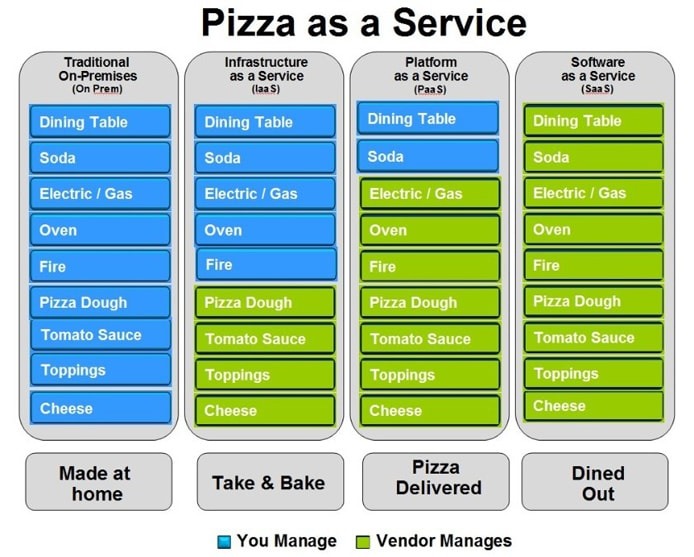
src: http://bigcommerce.com
[Avg. reading time: 7 minutes]
Challenges of Cloud Computing
Privacy:
Cloud and Big Data often involve sensitive information such as addresses, credit card details, and social security numbers. It is crucial for users and organizations to implement proper security measures, such as encryption, access controls, and regular audits, to protect this data from unauthorized access and breaches.
Compliance:
Cloud providers often replicate data across multiple regions to ensure availability and resilience. However, this can conflict with compliance requirements, such as data residency regulations that mandate data must not leave a specific geographic location or organization. For example, some regulations prevent storing data outside a specific country or within certain geopolitical regions.
Example: Google Cloud Platform (GCP) does not have data centers in mainland China, which could affect businesses operating under data sovereignty laws in that region.
Data Availability:
Cloud services rely on internet connectivity and speed, making them susceptible to interruptions in service due to network issues. The choice of cloud provider significantly impacts data availability, as providers like AWS, GCP, and Azure offer extensive global networks with redundancy and backup capabilities to ensure high availability and reliability.
Connectivity:
The performance of cloud services is highly dependent on the availability and speed of the internet connection. Poor connectivity can lead to latency issues, slower access to services, and potential downtime, impacting the user experience and business operations.
Vendor Lock-In:
Cloud services often involve proprietary tools, APIs, and platforms that can create vendor lock-in, making it challenging to switch providers without incurring significant costs or re-engineering efforts. This can limit flexibility and potentially increase long-term costs.
Data Transfer Costs:
Moving data in and out of the cloud can incur significant costs, particularly with large datasets or frequent transfers. Understanding the pricing models and optimizing data transfer strategies is essential to managing expenses effectively.
Limited Control and Flexibility:
Cloud providers manage the underlying infrastructure, which means users have limited control over the environment. This can impact performance tuning, custom configurations, and specific requirements that might not be fully supported by the provider’s managed services.
[Avg. reading time: 4 minutes]
High Availability
High Availability can also be called Uptime. Refers to the accessibility of a system that can operate without any interruptions for an extended period.
What’s the difference between the following?
- 99%
- 99.9%
- 99.99%
- 99.999%
Availability Levels and Downtime
99% Availability (Two Nines):
- Downtime: ~3.65 days per year
- Monthly Downtime: ~7.2 hours
- This level is common for non-critical systems where some downtime is tolerable.
99.9% Availability (Three Nines):
- Downtime: ~8.76 hours per year
- Monthly Downtime: ~43.8 minutes
- Suitable for many business applications with occasional tolerance for downtime.
99.99% Availability (Four Nines):
- Downtime: ~52.6 minutes per year
- Monthly Downtime: ~4.38 minutes
- Often used for critical applications where downtime can have significant business impacts.
99.999% Availability (Five Nines):
- Downtime: ~5.26 minutes per year
- Monthly Downtime: ~26.3 seconds
- Known as “five nines,” this level is aimed at highly critical systems, such as those in healthcare, finance, or telecommunications, where even a few minutes of downtime is unacceptable.
As per the Gartner survey, it costs $5,600 per minute.
https://blogs.gartner.com/andrew-lerner/2014/07/16/the-cost-of-downtime/
[Avg. reading time: 4 minutes]
Azure Cloud
Servers: Individual Machines
Data Centers: These are the physical buildings that house servers and other components like networking, storage, and compute resources
Availability Zones: Each Availability Zone comprises one or more data centers. Availability Zones are tolerant to data center failures through redundancy and logical isolation of services.
Regions: Regions are typically located in different geographic areas and can be selected to keep data and applications close to users.
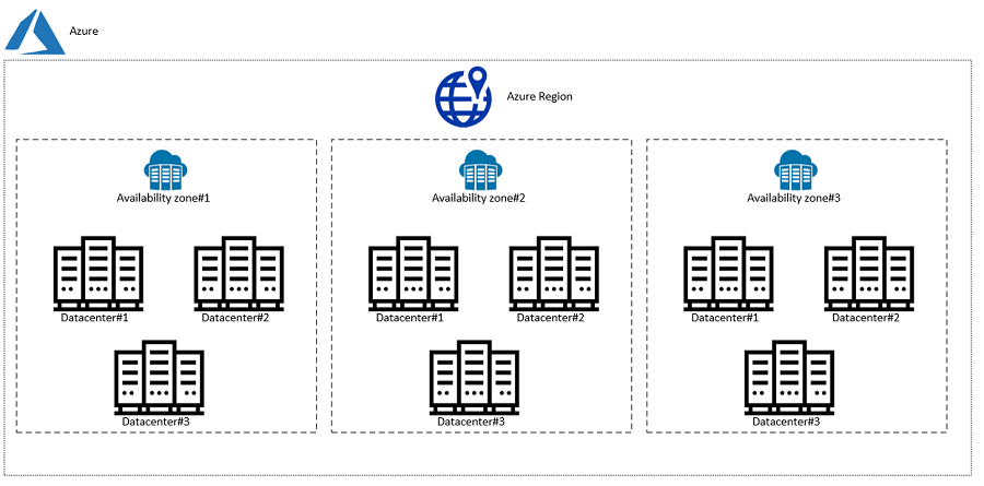
Source: https://www.unixarena.com/2020/08/what-is-the-availablity-zone-on-azure.html
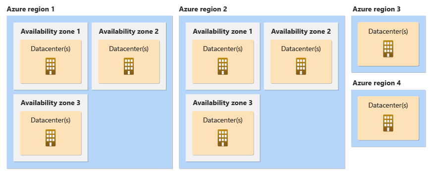
Source: https://learn.microsoft.com/en-us/azure/reliability/availability-zones-overview?tabs=azure-cli
Paired Regions: Paired regions support certain types of multi-region deployment approaches.
Paired regions are physically separated by at least 300 miles, reducing the likelihood that a natural disaster or large-scale infrastructure failure would affect both regions.
Geo-Redundant Storage: Data replicated with GRS will be stored in the primary region and replicated in the secondary paired region.
Site Recovery: Azure Site Recovery services enable failover to the paired region in the event of a major outage.
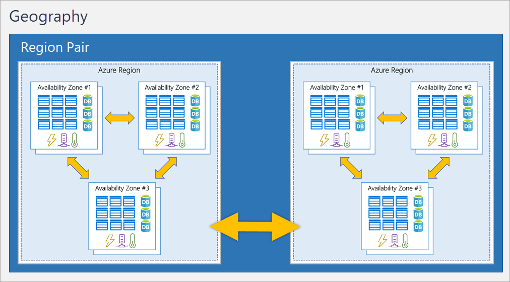
Source: https://i.stack.imgur.com/BwHct.png
[Avg. reading time: 15 minutes]
Services
Azure Core Services
Compute
Azure Virtual Machines (IaaS)
- Windows and Linux VMs
- Flexible sizing and scaling options
- Support for specialized workloads (GPU, HPC)
Azure App Service (PaaS)
- Web Apps, API Apps, Mobile Apps
- Managed platform for hosting applications
- Auto-scaling and deployment options
Azure Functions (Serverless)
- Event-driven compute platform
- Pay-per-execution pricing
- Automatic scaling
Azure Container Instances and Azure Kubernetes Service (AKS)
- Containerized application deployment
- Managed Kubernetes orchestration
- Microservices architecture support
Storage
Azure Blob Storage
- Object storage for unstructured data
- Hot, cool, and archive tiers
- Scalable and cost-effective
Azure Data Lake Storage Gen2 (ADLS Gen2)
- Hierarchical namespace for file organization
- Built on Azure Blob Storage
- Optimized for big data analytics
- Fine-grained ACLs (Access Control Lists)
- Cost-effective storage for large-scale data analytics
- Support for both structured and unstructured data
Azure Files
- Fully managed file shares
- SMB and REST protocols
- Hybrid storage solutions
Azure Disk Storage
- Block-level storage volumes
- Ultra disks, Premium SSD, Standard SSD, Standard HDD
- VM-attached storage
General Features
| Feature | Azure Blob Storage | ADLS Gen2 |
|---|---|---|
| Primary Use Case | General purpose object storage | Big data analytics |
| Namespace Structure | Flat namespace | Hierarchical namespace |
| Cost | Lower cost for basic operations | Higher cost, optimized for analytics |
| Security | Basic security model | POSIX-compliant ACLs |
| Performance | Optimized for high transaction rates | Optimized for high-throughput analytics |
| Scalability | Petabyte scale | Exabyte scale |
Use Cases
| Scenario | Azure Blob Storage | ADLS Gen2 |
|---|---|---|
| Static Website Hosting | ✓ Ideal | ✗ Not recommended |
| Media Streaming | ✓ Ideal | ✗ Not optimal |
| Backup & Archive | ✓ Cost-effective | ✗ Expensive |
| Data Lake | ✗ Limited capabilities | ✓ Ideal |
| Hadoop Workloads | ✗ Not optimal | ✓ Native support |
| Real-time Analytics | ✗ Limited | ✓ Optimized |
Integration & Compatibility
| Service/Feature | Azure Blob Storage | ADLS Gen2 |
|---|---|---|
| Azure CDN | ✓ Native support | ⚠ Possible but complex |
| Azure Synapse | ⚠ Basic support | ✓ Native integration |
| HDInsight | ⚠ Limited support | ✓ Native support |
| Hadoop Compatible | ✗ No | ✓ Yes |
| Power BI | ⚠ Basic support | ✓ Enhanced support |
Performance Characteristics
| Operation Type | Azure Blob Storage | ADLS Gen2 |
|---|---|---|
| Small File Operations | ✓ Optimized | ⚠ Not optimal |
| Large File Operations | ⚠ Basic performance | ✓ Optimized |
| Random Access | ✓ Good | ⚠ Limited |
| Sequential Access | ⚠ Basic | ✓ Optimized |
| Directory Operations | ✗ N/A | ✓ Efficient |
Security & Governance
| Feature | Azure Blob Storage | ADLS Gen2 |
|---|---|---|
| Azure AD Integration | ✓ Basic | ✓ Enhanced |
| POSIX ACLs | ✗ No | ✓ Yes |
| Folder-level Security | ✗ No | ✓ Yes |
| Audit Logging | ⚠ Basic | ✓ Enhanced |
| Data Lifecycle Management | ✓ Yes | ✓ Yes |
Azure Table Storage
- NoSQL key-value store
- Schema-less design
- Cost-effective storage for structured datas
Networking
Azure Virtual Network (VNet)
- Isolated network environment
- Subnet configuration
- Network security groups (NSGs)
Azure Load Balancer
- Traffic distribution
- High availability
- Layer 4 (TCP/UDP) load balancing
Azure Application Gateway
- Web traffic load balancer
- SSL termination
- Web application firewall (WAF)
Azure ExpressRoute
- Private connectivity to Azure
- Bypasses public internet
- Higher reliability and lower latency
Identity and Access Management
Azure Active Directory (Azure AD)
- Cloud-based identity service
- Single Sign-On (SSO)
- Multi-Factor Authentication (MFA)
Role-Based Access Control (RBAC)
- Fine-grained access management
- Custom role definitions
- Resource-level permissions
Managed Identities
- Automatic credential management
- Service-to-service authentication
- Enhanced security without stored credentials
Monitoring & Management Services
Azure Monitor
- Platform metrics and logs
- Application insights
- Real-time monitoring
Azure Resource Manager
- Deployment and management
- Resource organization
- Access control and auditing
Azure Backup
- Cloud-based backup solution
- VM, database, and file backup
- Long-term retention
Azure Site Recovery
- Disaster recovery service
- Business continuity
- Automated replication and failover
Security Services
Azure Security Center
- Unified security management
- Threat protection
- Security posture assessment
Azure Key Vault
- Secret management
- Key management
- Certificate management
Azure DDoS Protection
- Network protection
- Automatic attack mitigation
- Real-time metrics and reporting
Azure Sentinel
- Cloud-native SIEM
- AI-powered threat detection
- Security orchestration and automation
DevOps in Azure
Azure DevOps
- Source control (Azure Repos)
- CI/CD pipelines
- Project management (Azure Boards)
Azure Artifacts
- Package management
- Integrated dependency tracking
- Secure artifact storage
Azure Test Plans
- Manual and exploratory testing
- Test case management
- User acceptance testing
GitHub Integration
- GitHub Actions support
- Repository management
- Code collaboration tools
Terms to knows
Subscription
- Logical container associated with a particular Azure account.
- Different subscriptions for various groups within company.
Example: Meta -> Facebook, Instagram, Whatsapp, Oculus
Key Aspects
- Billing and Payment
- Access Control at high level
- Service Availability across Regions (US East, Asia, EU West)
- Governance Compliance and Policies
Resource Group
Container that holds related resources for an Azure solution.
- Project Based Organization
- All resources for a specific project
- Environment Based
- Dev, QA, UAT, Prod
Key Aspects
- Resources in a group share same lifecycle
- Inherited permissions to resources
- Track expenses by resource group
Best Practices
- Use consistent naming conventions
- Apply appropriate tags
- Implement least privilege access
- Regular resource group auditing
- Consider geographic location for resources
[Avg. reading time: 10 minutes]
Storages
Azure Blob Storage
-
Blob storage is designed for storing large amounts of unstructured data, such as images, videos, backups, log files, and other binary data.
-
It provides three different access tiers: Hot (frequently accessed data), Cool (infrequently accessed data), and Archive (rarely accessed data).
-
Blob storage offers high scalability, availability, and durability.
Example: A media streaming service can store video files, audio files, and images in Blob storage. The files can be accessed from anywhere and served to users on various devices.
Azure Data Lake Storage
-
Data Lake Storage is a secure, scalable, and massively parallel data storage service optimized for big data analytics workloads.
-
It supports storing and processing structured, semi-structured, and unstructured data in a single location.
-
Azure Data Lake Storage integrates with Azure HDInsight, Azure Databricks, and other big data analytics services.
Example: Best suited for storing Data files such as csv, parquet. As it offers hierarchical namespace to store folders and files. Economical and offers path based syntax (abfss://conatiner@storage/folder/file.csv)
Azure Table Storage
-
Table storage is a NoSQL key-value store designed for storing semi-structured data.
-
It provides a schemaless design, allowing you to store heterogeneous data types.
-
Table storage is suitable for storing structured, non-relational data with massive scale and low-cost storage.
Example: A mobile application can store user profiles, preferences, and other structured data in Azure Table Storage. The schemaless design of Table Storage allows for flexible data modeling and easy scalability as the application grows.
Azure Disk Storage
-
Disk storage provides persistent storage for Azure Virtual Machines (VMs).
-
It offers different disk types, such as Ultra Disks, Premium SSDs, Standard SSDs, and Standard HDDs, to meet various performance and cost requirements.
-
Disk storage is used for operating system disks, data disks, and temporary disks for Azure VMs.
Example: An e-commerce website can use Azure Disk Storage to store the operating system disks and data disks for the virtual machines running the web application and database servers.
Azure File Storage
-
File storage provides fully managed file shares that can be mounted and accessed like a regular file system.
-
It allows you to share files between virtual machines (VMs), applications, and on-premises deployments.
-
Azure File Storage supports the Server Message Block (SMB) protocol and Network File System (NFS) protocol.
Example: A development team can create a file share using Azure File Storage to store and share source code, documentation, and other project files. The file share can be accessed concurrently by multiple team members, regardless of their location.
Azure Queue Storage
-
Queue storage is a messaging service that enables you to store and retrieve messages in a queue.
-
It is commonly used for building reliable and scalable cloud-based applications and services.
-
Messages can be processed asynchronously, enabling decoupled communication between components.
Example: A web application can use Azure Queue Storage to offload resource-intensive tasks, such as image processing or sending email notifications, to a queue.
#azure #adls #storageaccount #containers
[Avg. reading time: 7 minutes]
Demo
- Subscription
- Create a new Resource Group
- EntraID
- Create a VM
https://learn.microsoft.com/en-us/azure/virtual-machines/windows/quick-create-portal
Azure CLI
https://learn.microsoft.com/en-us/cli/azure/install-azure-cli
Azure Login
az login
Azure Group
az group list --output table
# Create a new Resource Group
az group create --name resgroup_via_cli --location eastus2
# delete the Resource Group
az group delete --name resgroup_via_cli
# Delete the Resource Group without Prompt
az group delete --name resgroup_via_cli -y
Azure VM
# List all VMs.
az vm list
# Azure List Sizes
az vm list-sizes --location eastus
az vm list-sizes --location eastus --output table
az vm list-sizes --location eastus --query "[].{AccountName:name, Cores:numberOfCores}" --output table
az vm list-sizes --location eastus | jq -r 'sort_by([.numberOfCores,.maxDataDiskCount]) | .[] | "\(.name) \(.numberOfCores) \(.memoryInMB)MB \(.osDiskSizeInMB)MB \(.resourceDiskSizeInMB)MB \(.maxDataDiskCount)"'
az vm create --resource-group resgroup_via_cli --name myubuntu --image Ubuntu2204 --generate-ssh-keys
az vm show --resource-group resgroup_via_cli --name myubuntu --query "{username:osProfile.adminUsername}" --output tsv
az vm list-ip-addresses --resource-group resgroup_via_cli --name myubuntu
az vm show --resource-group resgroup_via_cli --name myubuntu --query "hardwareProfile.vmSize" --output tsv
# Start a VM:
az vm start --resource-group resgroup_via_cli --name myubuntu
# Stop a VM:
az vm stop --resource-group resgroup_via_cli --name myubuntu
# Deallocate a VM
az vm deallocate --resource-group resgroup_via_cli --name myubuntu
az vm resize -g resgroup_via_cli -n myubuntu --size Standard_DS3_v2
# Resize all VMs in a resource group.
az vm resize --size Standard_DS3_v2 --ids $(az vm list -g resgroup_via_cli --query "[].id" -o
tsv)
# Delete a VM
az vm delete --resource-group resgroup_via_cli --name myubuntu
Azure Storage
az storage account list -g gc-resourcegroup --output table
az storage account list --resource-group gc-resourcegroup --query "[].{AccountName:name, Location:location}" --output table
az storage account show-connection-string --name gcstorage007 -g gc-resourcegroup
# Create a storage account:
az storage account create --name newstorage --resource-group MyResourceGroup --location eastus --sku Standard_LRS
[Avg. reading time: 23 minutes]
Terraform
Features of Terraform
Infrastructure as Code: Terraform allows you to write, plan, and create infrastructure using configuration files. This makes infrastructure management automated, consistent, and easy to collaborate on.
Multi-Cloud Support: Terraform supports many cloud providers and on-premises environments, allowing you to manage resources across different platforms seamlessly.
State Management: Terraform keeps track of the current state of your infrastructure in a state file. This enables you to manage changes, plan updates, and maintain consistency in your infrastructure.
Resource Graph: Terraform builds a resource dependency graph that helps in efficiently creating or modifying resources in parallel, speeding up the provisioning process and ensuring dependencies are handled correctly.
Immutable Infrastructure: Terraform promotes the practice of immutable infrastructure, meaning that resources are replaced rather than updated directly. This ensures consistency and reduces configuration drift.
Execution Plan: Terraform provides an execution plan (terraform plan) that previews changes before they are applied, allowing you to understand and validate the impact of changes before implementing them.
Modules: Terraform supports reusability through modules, which are self-contained, reusable pieces of configuration that help you maintain best practices and reduce redundancy in your infrastructure code.
Community and Ecosystem: Terraform has a large open-source community and many providers and modules available through the Terraform Registry, which makes it easier to get started and integrate with various services.
Use Cases
- Multi-Cloud Provisioning
- Infrastructure Scaling
- Disaster Recovery
- Environment Management
- Compliance & Standardization
- CI/CD Pipelines
- Speed and Simplicity
- Team Collaboration
- Error Reduction
- Enhanced Security
Install Terraform CLI
<a href="https://developer.hashicorp.com/terraform/downloads"" title="" target="_blank">Terraform Download
Terraform Structure for Azure
Provider Block: Specifies Azure as the cloud provider and authentication method.
provider "azurerm" {
features {}
subscription_id = "your-subscription-id"
tenant_id = "your-tenant-id"
}
Resource Block: Defines Azure resources like VMs, Storage Accounts, or Virtual Networks.
resource "azurerm_virtual_machine" "example" {
name = "example-vm"
location = "East US"
resource_group_name = azurerm_resource_group.example.name
vm_size = "Standard_DS1_v2"
storage_image_reference {
publisher = "Canonical"
offer = "UbuntuServer"
sku = "18.04-LTS"
version = "latest"
}
}
Data Block: Retrieves information about existing Azure resources.
data "azurerm_resource_group" "example" {
name = "existing-resource-group"
}
data "azurerm_virtual_network" "existing" {
name = "existing-vnet"
resource_group_name = data.azurerm_resource_group.example.name
}
Variable Block: Defines input variables for flexible configuration.
variable "location" {
description = "The Azure Region to deploy resources"
type = string
default = "East US"
}
variable "environment" {
description = "Environment name"
type = string
default = "dev"
}
Output Block: Returns values after applying the configuration.
output "vm_ip_address" {
value = azurerm_public_ip.example.ip_address
}
output "storage_account_primary_key" {
value = azurerm_storage_account.example.primary_access_key
sensitive = true
}
Module Block: Reusable components for Azure infrastructure.
module "vnet" {
source = "./modules/vnet"
resource_group_name = azurerm_resource_group.example.name
location = var.location
address_space = ["10.0.0.0/16"]
}
Locals Block: Local variables for repeated values.
locals {
common_tags = {
Environment = var.environment
Project = "MyProject"
Owner = "DevOps Team"
}
resource_prefix = "${var.environment}-${var.location}"
}
az login
Get the Subscription ID
Create a new folder
Copy the .tf into it
storage.tf
terraform {
required_providers {
azurerm = {
source = "hashicorp/azurerm"
version = "=4.4.0"
}
}
}
provider "azurerm" {
features{
}
subscription_id = "your subscription id"
}
# Create a resource group
resource "azurerm_resource_group" "example" {
name = "demo-resourcegroup-via-tf"
location = "East US"
tags = {
environment = "dev"
}
}
# Create a storage account
resource "azurerm_storage_account" "example" {
name = "chandr34demo"
resource_group_name = azurerm_resource_group.example.name
location = azurerm_resource_group.example.location
account_tier = "Standard"
account_replication_type = "LRS"
tags = {
environment = "dev"
}
}
terraform init
terraform validate
terraform plan
terraform apply
terraform destroy
Repeat the above steps to create Resource Group, Blob, ADLS, Containers
Remember to install Azure CLI.
az login
# Configure the Azure provider
terraform {
required_providers {
azurerm = {
source = "hashicorp/azurerm"
version = "= 4.4.0"
}
}
}
# Configure the Microsoft Azure Provider using CLI authentication
provider "azurerm" {
features {}
subscription_id = "your subscription id"
}
# Create a resource group
resource "azurerm_resource_group" "example" {
name = "gc-example-resources"
location = "East US"
tags = {
environment = "dev"
}
}
# Create a storage account with ADLS Gen2 enabled
resource "azurerm_storage_account" "adls" {
name = "chandr34adlsgen2"
resource_group_name = azurerm_resource_group.example.name
location = azurerm_resource_group.example.location
account_tier = "Standard"
account_replication_type = "LRS"
account_kind = "StorageV2" # Required for ADLS Gen2
is_hns_enabled = true # This enables hierarchical namespace for ADLS Gen2
tags = {
environment = "dev"
type = "data-lake"
}
}
# Create a storage account for Blob storage
resource "azurerm_storage_account" "blob" {
name = "chandr34blobstorage"
resource_group_name = azurerm_resource_group.example.name
location = azurerm_resource_group.example.location
account_tier = "Standard"
account_replication_type = "LRS"
account_kind = "StorageV2"
is_hns_enabled = false # Disabled for regular blob storage
# Enable blob-specific features
blob_properties {
versioning_enabled = true
last_access_time_enabled = true
container_delete_retention_policy {
days = 7
}
}
tags = {
environment = "dev"
type = "blob"
}
}
# Create a container in the blob storage account
resource "azurerm_storage_container" "blob_container" {
name = "myblobs"
storage_account_name = azurerm_storage_account.blob.name
container_access_type = "private"
}
# Create a filesystem in the ADLS Gen2 storage account
resource "azurerm_storage_data_lake_gen2_filesystem" "example" {
name = "myfilesystem"
storage_account_id = azurerm_storage_account.adls.id
}
Create a Linux VM with SSH Keys
Create a new folder and continue
vm_ssh.tf
# Provider configuration
terraform {
required_providers {
azurerm = {
source = "hashicorp/azurerm"
version = "= 4.4.0"
}
tls = {
source = "hashicorp/tls"
version = "~> 4.0"
}
local = {
source = "hashicorp/local"
version = "~> 2.0"
}
}
}
provider "azurerm" {
features {}
subscription_id = "your subscription id"
}
# Generate SSH key
resource "tls_private_key" "ssh" {
algorithm = "RSA"
rsa_bits = 4096
}
# Save private key locally
resource "local_file" "private_key" {
content = tls_private_key.ssh.private_key_pem
filename = "vm_ssh_key.pem"
file_permission = "0600"
}
# Resource Group
resource "azurerm_resource_group" "rg" {
name = "ubuntu-vm-rg"
location = "eastus"
}
# Virtual Network
resource "azurerm_virtual_network" "vnet" {
name = "ubuntu-vm-vnet"
resource_group_name = azurerm_resource_group.rg.name
location = azurerm_resource_group.rg.location
address_space = ["10.0.0.0/16"]
}
# Subnet
resource "azurerm_subnet" "subnet" {
name = "ubuntu-vm-subnet"
resource_group_name = azurerm_resource_group.rg.name
virtual_network_name = azurerm_virtual_network.vnet.name
address_prefixes = ["10.0.1.0/24"]
}
# Public IP
resource "azurerm_public_ip" "pip" {
name = "ubuntu-vm-pip"
resource_group_name = azurerm_resource_group.rg.name
location = azurerm_resource_group.rg.location
allocation_method = "Static"
sku = "Standard"
}
# Network Security Group
resource "azurerm_network_security_group" "nsg" {
name = "ubuntu-vm-nsg"
resource_group_name = azurerm_resource_group.rg.name
location = azurerm_resource_group.rg.location
security_rule {
name = "SSH"
priority = 1001
direction = "Inbound"
access = "Allow"
protocol = "Tcp"
source_port_range = "*"
destination_port_range = "22"
source_address_prefix = "*"
destination_address_prefix = "*"
}
}
# Network Interface
resource "azurerm_network_interface" "nic" {
name = "ubuntu-vm-nic"
resource_group_name = azurerm_resource_group.rg.name
location = azurerm_resource_group.rg.location
ip_configuration {
name = "internal"
subnet_id = azurerm_subnet.subnet.id
private_ip_address_allocation = "Dynamic"
public_ip_address_id = azurerm_public_ip.pip.id
}
}
# Connect the NSG to the subnet
resource "azurerm_subnet_network_security_group_association" "nsg_association" {
subnet_id = azurerm_subnet.subnet.id
network_security_group_id = azurerm_network_security_group.nsg.id
}
# Virtual Machine
resource "azurerm_linux_virtual_machine" "vm" {
name = "ubuntu-vm"
resource_group_name = azurerm_resource_group.rg.name
location = azurerm_resource_group.rg.location
size = "Standard_D2s_v3"
admin_username = "azureuser"
network_interface_ids = [
azurerm_network_interface.nic.id
]
admin_ssh_key {
username = "azureuser"
public_key = tls_private_key.ssh.public_key_openssh
}
os_disk {
caching = "ReadWrite"
storage_account_type = "Standard_LRS"
}
source_image_reference {
publisher = "Canonical"
offer = "0001-com-ubuntu-server-jammy"
sku = "22_04-lts"
version = "latest"
}
}
# Outputs
output "public_ip_address" {
value = azurerm_public_ip.pip.ip_address
}
output "ssh_command" {
value = "ssh -i vm_ssh_key.pem azureuser@${azurerm_public_ip.pip.ip_address}"
}
output "tls_private_key" {
value = tls_private_key.ssh.private_key_pem
sensitive = true
}
ssh aazureuser@ip
Create a Linux VM with UserName and PWD
Create a new folder and continue
vm_pwd.tf
# Provider configuration
terraform {
required_providers {
azurerm = {
source = "hashicorp/azurerm"
version = "= 4.4.0"
}
}
}
provider "azurerm" {
features {}
subscription_id = "your subscription id"
}
# Resource Group
resource "azurerm_resource_group" "rg" {
name = "ubuntu-vm-rg"
location = "eastus"
}
# Virtual Network
resource "azurerm_virtual_network" "vnet" {
name = "ubuntu-vm-vnet"
resource_group_name = azurerm_resource_group.rg.name
location = azurerm_resource_group.rg.location
address_space = ["10.0.0.0/16"]
}
# Subnet
resource "azurerm_subnet" "subnet" {
name = "ubuntu-vm-subnet"
resource_group_name = azurerm_resource_group.rg.name
virtual_network_name = azurerm_virtual_network.vnet.name
address_prefixes = ["10.0.1.0/24"]
}
# Public IP
resource "azurerm_public_ip" "pip" {
name = "ubuntu-vm-pip"
resource_group_name = azurerm_resource_group.rg.name
location = azurerm_resource_group.rg.location
allocation_method = "Static"
sku = "Standard"
}
# Network Security Group
resource "azurerm_network_security_group" "nsg" {
name = "ubuntu-vm-nsg"
resource_group_name = azurerm_resource_group.rg.name
location = azurerm_resource_group.rg.location
security_rule {
name = "SSH"
priority = 1001
direction = "Inbound"
access = "Allow"
protocol = "Tcp"
source_port_range = "*"
destination_port_range = "22"
source_address_prefix = "*"
destination_address_prefix = "*"
}
}
# Network Interface
resource "azurerm_network_interface" "nic" {
name = "ubuntu-vm-nic"
resource_group_name = azurerm_resource_group.rg.name
location = azurerm_resource_group.rg.location
ip_configuration {
name = "internal"
subnet_id = azurerm_subnet.subnet.id
private_ip_address_allocation = "Dynamic"
public_ip_address_id = azurerm_public_ip.pip.id
}
}
# Connect the NSG to the subnet
resource "azurerm_subnet_network_security_group_association" "nsg_association" {
subnet_id = azurerm_subnet.subnet.id
network_security_group_id = azurerm_network_security_group.nsg.id
}
# Virtual Machine
resource "azurerm_linux_virtual_machine" "vm" {
name = "ubuntu-vm"
resource_group_name = azurerm_resource_group.rg.name
location = azurerm_resource_group.rg.location
size = "Standard_D2s_v3"
admin_username = "azureuser"
admin_password = "H3ll0W0rld$"
disable_password_authentication = false
network_interface_ids = [
azurerm_network_interface.nic.id
]
os_disk {
caching = "ReadWrite"
storage_account_type = "Standard_LRS"
}
source_image_reference {
publisher = "Canonical"
offer = "0001-com-ubuntu-server-jammy"
sku = "22_04-lts"
version = "latest"
}
}
# Output the public IP
output "public_ip_address" {
value = azurerm_public_ip.pip.ip_address
}
[Avg. reading time: 1 minute]
Data Engineering
- Batch vs Streaming
- Kafka
- Quality & Governance
- Medallion Architecture
- Data Engineering Model
- Data Mesh
[Avg. reading time: 8 minutes]
Batch vs Streaming
Batch Processing
Batch means collect first, process later.
- Works on large chunks of accumulated data
- High throughput, cheaper, simpler
- Results are not real-time
- Typically minutes, hours, or days delayed
Examples:
- Daily or weekly sales reports
- End-of-day stock portfolio reconciliation
- Monthly billing cycles
- ETL pipelines that refresh a data warehouse
Use cases
- Data does not need to be acted on immediately
- A few minutes or hours of delay is acceptable
- You’re cleaning, transforming, aggregating large datasets
Stream Processing
Streaming means process events the moment they arrive.
- Low-latency (milliseconds to seconds)
- Continuous, event-by-event processing
- Ideal for real-time analytics and alerting
- Stateful systems maintain event history or running context
Examples:
- Stock price updates
- Fraud detection for credit cards
- Real-time gaming leaderboards
- IoT sensor monitoring
Use cases
- You need instant reactions
- Delays cause risk, loss, or bad UX
Micro Batch
Micro-batching groups incoming events into tiny batches and processes each mini-batch as a unit, giving near real-time outputs without true event-by-event streaming.
Micro-batch is not full streaming, and not full batch.
It’s a hybrid model where data is processed in very small batches at very short intervals (usually 100 ms to a few seconds).
Batch processing, but done so frequently that it feels like streaming.
Example: Realtime vs Microbatch
Credit Card Fraud Detection (Realtime)
Fraud scoring must be event-by-event or at worst sub-second.
- The bank must decide immediately: approve or decline
- Customer is standing at a checkout counter
- Delay = blocked transaction or fraud slipping through
- Regulatory requirements often demand immediate response
Credit Card Payment Posting (Micro Batch)
When a customer makes a payment toward their balance (online, app, ACH, etc), updating the backend systems does not require millisecond consistency.
Even if the balance updates with a 1-minute delay:
- No fraud risk
- No UX problem
- No operational impact
+------------------------------+
| STREAMING |
| Event → Process → Output |
| Latency: milliseconds |
+------------------------------+
+------------------------------+
| MICRO-BATCH |
| Tiny windows → Process |
| Latency: 0.5–10 seconds |
+------------------------------+
+------------------------------+
| BATCH |
| Accumulate → Process |
| Latency: minutes–hours |
+------------------------------+
Why Redis Pub/Sub is NOT real streaming
Redis Pub/Sub is often mistaken as “streaming”, but:
- Messages are not persisted
- No replay capability
- No consumer groups
- No fault tolerance
- If a subscriber goes offline — the message is gone
Use cases
- Lightweight notifications
- Chat-like message passing
- Ephemeral real-time signals
Not suitable
- Analytics
- Compliance or auditing
- Durable event logs
- Replaying data
- Multi-consumer systems
[Avg. reading time: 27 minutes]
Kafka
Introduction
Apache Kafka is a distributed streaming platform designed for high-throughput, fault-tolerant, real-time data pipelines. Its a publish-subscribe messaging system that excels at handling real-time data streams.
- Built at LinkedIn, open-sourced in 2011
- Designed as a distributed commit log
- Handles millions of events per second
- Extremely scalable and fault-tolerant
- Stores data durably for replay
Key Features
- High throughput: Can handle millions of messages per second
- Fault-tolerant: Data is replicated across servers
- Scalable: Can easily scale horizontally across multiple servers
- Persistent storage: Keeps messages for as long as you need
Apache Kafka is a publish/subscribe messaging system designed to solve this problem. It is often described as a “distributed commit log” or, more recently, as a “distributing streaming platform.”
A filesystem or database commit log is designed to provide a durable record of all transactions so that they can be replayed to build the state of a system consistently.
Basic Terms
Topic
Think of it like a TV Channel or Radio station where messages are published. A category or feed name to which messages are stored and published.
Key characteristics
- Multi-subscriber (multiple consumers can read from same topic)
- Durable (messages are persisted based on retention policy)
- Ordered (within each partition)
- Like a database table, but with infinite append-only logs
Messages
- The fundamental unit of data in Kafka
- Similar to a row in a database, but immutable (can’t be changed once written)
Structure of a message
- Value: The actual data payload (array of bytes)
- Key: Optional identifier (more on this below)
- Timestamp
- Optional metadata (headers)
Messages don’t have a specific format requirement - they’re just bytes.
Sample Message
+-------------------------------------------------------------+
| Kafka Record |
+-------------------------------------------------------------+
| Key (bytes) | Optional. Used for partitioning |
+-------------------------------------------------------------+
| Value (bytes) | Actual payload (JSON/Avro/Proto…) |
+-------------------------------------------------------------+
| Timestamp | CreateTime or LogAppendTime |
+-------------------------------------------------------------+
| Headers (optional) | Arbitrary metadata (byte key/value)|
+-------------------------------------------------------------+
| Topic | Logical stream name |
+-------------------------------------------------------------+
| Partition | Defines ordering and parallelism |
+-------------------------------------------------------------+
| Offset | Sequential id within the partition |
+-------------------------------------------------------------+
When the Producer sends
{
"key": "user_123",
"value": {
"userId": "user_123",
"action": "login",
"device": "iPhone",
"location": "New York"
},
"headers": {
"traceId": "abc-123-xyz",
"version": "1.0",
"source": "mobile-app"
}
}
consumer receives
{
"topic": "user_activities",
"partition": 2,
"offset": 15,
"timestamp": "2024-11-13T14:30:00.123Z",
"key": "user_123",
"value": {
"userId": "user_123",
"action": "login",
"device": "iPhone",
"location": "New York"
},
"headers": {
"traceId": "abc-123-xyz",
"version": "1.0",
"source": "mobile-app"
}
}
Partitions
- Topics are broken down into multiple partitions
- Messages are written in an append-only fashion
Important aspects
- Each partition is an ordered, immutable sequence of messages
- Messages get a sequential ID called an “offset” within their partition
- Time-ordering is guaranteed only within a single partition, not across the entire topic
- Provides redundancy and scalability
- Can be hosted on different servers
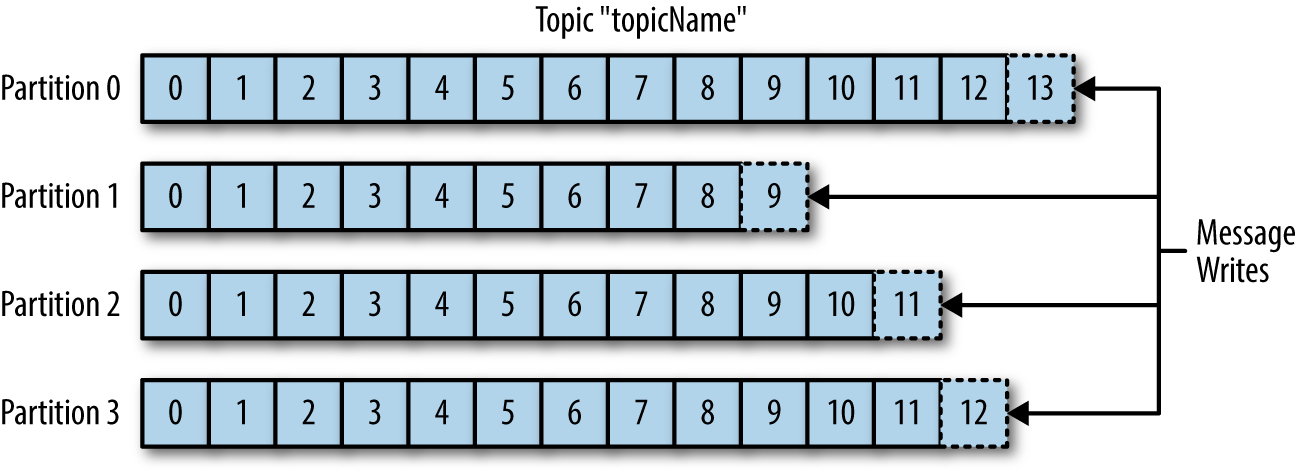
Keys
An optional identifier for messages serves two main purposes:**
Partition Determination:
- Messages with same key always go to same partition
- No key = round-robin distribution across partitions
- Uses formula: hash(key) % number_of_partitions
Data Organization:
- Groups related messages together
- Useful for message compaction
Real-world Example:
Topic: "user_posts"
Key: userId
Message: post content
Partitions: Multiple partitions for scalability
Result: All posts from the same user (same key) go to the same partition, maintaining order for that user's posts
Offset
A unique sequential identifier for messages within a partition, starts at 0 and increments by 1 for each message
Important characteristics:
- Immutable (never changes)
- Specific to a partition
- Used by consumers to track their position
- Example: In a partition with 5 messages → offsets are 0, 1, 2, 3, 4
Offset is a collaboration between Kafka and consumers:
- Kafka maintains offsets in a special internal topic called __consumer_offsets
This topic stores the latest committed offset for each partition per consumer group
Format in __consumer_offsets:
Key: (group.id, topic, partition)
Value: offset value
Two types of offsets for consumers:
- Current Position: The offset of the next message to be read
- Committed Offset: The last offset that has been saved to Kafka
Two types of Commits
- Auto Commit, default at a given interval in milli seconds.
- Manual Commit, done by consumer.
Batches
A collection of messages, all for the same topic and partition.
Benefits:
- More efficient network usage
- Better compression
- Faster I/O operations
Trade-off: Latency vs Throughput (larger batches = more latency but better throughput)
Producers
Producers create new messages. In general, a message will be produced on a specific topic.
Key behaviors:
- Can send to specific partitions or let Kafka handle distribution
Partition assignment happens through:
-
Round-robin (when no key is provided)
-
Hash of key (when message has a key)
-
Can specify acknowledgment requirements (acks)
Consumers and Consumer Groups
Consumers read messages from topics
Consumer Groups:
- Multiple consumers working together
- Each partition is read by ONLY ONE consumer in a group
- Automatic rebalancing if consumers join/leave the group
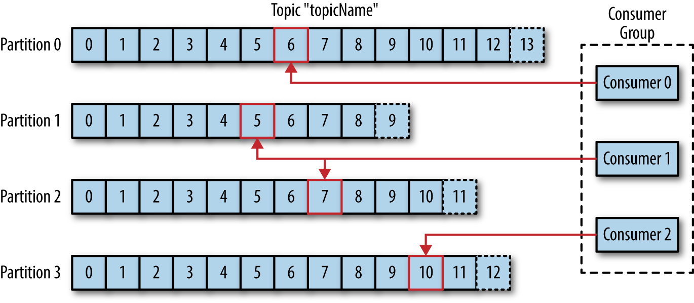
src: Oreilly Kafka Book
Brokers and Clusters
Broker:
Single Kafka server Responsibilities:
- Receive messages from producers
- Assign offsets
- Commit messages to storage
- Serve consumers
Cluster:
- Multiple brokers working together
- One broker acts as the Controller
- Handles replication and broker failure
- Provides scalability and fault tolerance
- A partition may be assigned to multiple brokers, which will result in Replication.
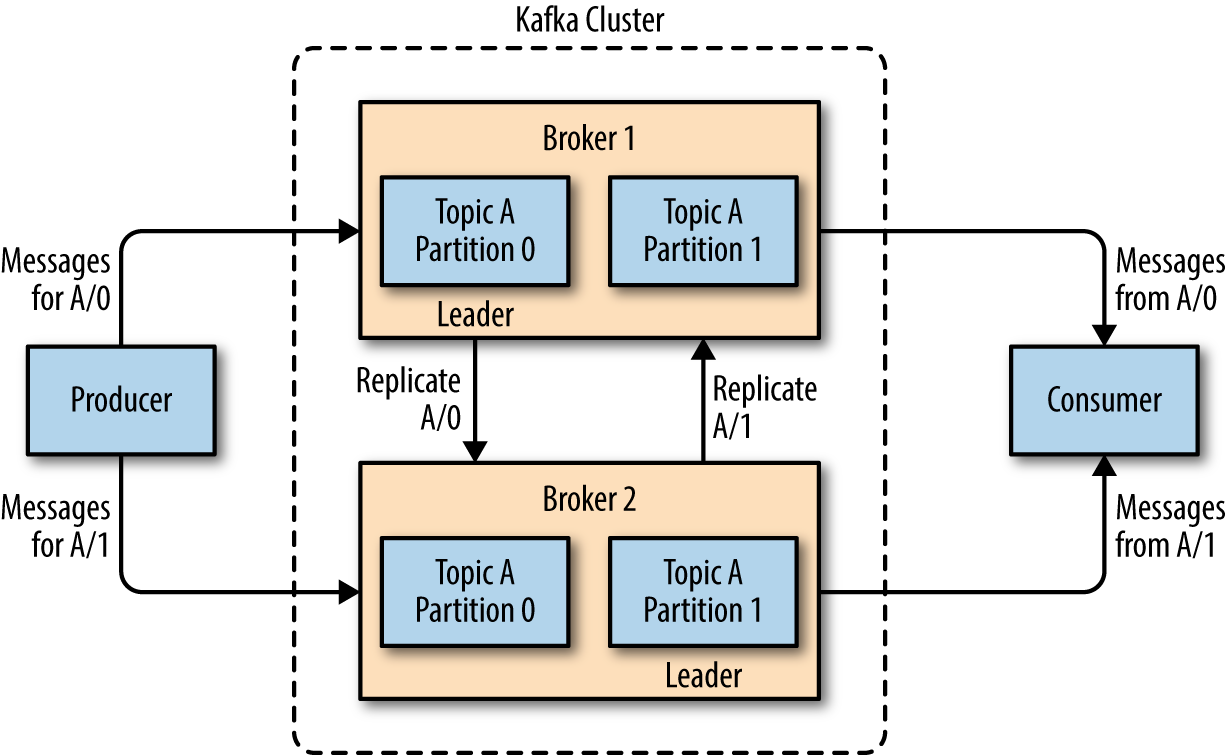
src: Oreilly Kafka Book
Message Delivery Semantics
Message Delivery Semantics are primarily controlled through Producer and Consumer configurations, not at the broker level.
At Least Once Delivery:
- Messages are never lost but might be redelivered.
- This is the default delivery method.
Scenario
- Consumer reads message
- Processes the message
- Crashes before committing offset
- After restart, reads same message again - retries > 0
Best for cases where duplicate processing is acceptable
from kafka import KafkaProducer
producer = KafkaProducer(
bootstrap_servers=['localhost:9092'],
acks='all', # Strong durability (optional but recommended)
retries=5, # Enables retry → allows duplicates
enable_idempotence=False # Required for at-least-once (duplicates allowed)
)
producer.send('events', b'sample message')
producer.flush()
Consumer
from kafka import KafkaConsumer
consumer = KafkaConsumer(
'events',
bootstrap_servers=['localhost:9092'],
group_id='my_group',
enable_auto_commit=False, # Manual commit required for at-least-once
auto_offset_reset='earliest'
)
for msg in consumer:
# Process the message
print(msg.value)
# Commit only AFTER processing — ensures at-least-once
consumer.commit()
At Most Once Delivery:
- Messages might be lost but never redelivered
- Commits offset as soon as message is received
- Use when some data loss is acceptable but duplicates are not - retry = 0
from kafka import KafkaProducer
producer = KafkaProducer(
bootstrap_servers=['localhost:9092'],
acks='all', # Strong durability (optional but recommended)
retries=0, # No Retry
enable_idempotence=False # Required for at-least-once (duplicates allowed)
)
producer.send('events', b'sample message')
producer.flush()
Consumer
enable_auto_commit=True auto_commit_interval_ms > 0
from kafka import KafkaConsumer
consumer = KafkaConsumer(
'events',
bootstrap_servers=['localhost:9092'],
group_id='my_group',
enable_auto_commit=True,
auto_offset_reset='earliest'
auto_commit_interval_ms=1000
)
for msg in consumer:
print(msg.value)
Exactly Once Delivery
- Messages are processed exactly once
- Achieved through transactional APIs
- Higher overhead but strongest guarantee - enable_idempotence=True
from kafka import KafkaProducer
producer = KafkaProducer(
bootstrap_servers=['localhost:9092'],
acks='all', # Must wait for all replicas
enable_idempotence=True, # Core requirement for EOS
retries=5, # Required (Kafka enforces this)
transactional_id='txn-1' # Required for transactions
)
# Initialize the transaction
producer.init_transactions()
# Start transaction
producer.begin_transaction()
# Send messages inside the transaction
producer.send('events', b'event one')
producer.send('events', b'event two')
# Commit transaction atomically
producer.commit_transaction()
Summary
- At Most Once: Highest performance, lowest reliability
- At Least Once: Good performance, possible duplicates
- Exactly Once: Highest reliability, lower performance
Can Producer and Consumer have different semantics? Like producer with Exactly Once and Consumer with Atleast Once?
Yes its possible.
# Producer with Exactly Once
exactly_once_producer = KafkaProducer(
bootstrap_servers=['localhost:9092'],
acks='all',
enable_idempotence=True,
transactional_id='prod-1'
)
# Consumer with At Least Once
at_least_once_consumer = KafkaConsumer(
'your_topic',
bootstrap_servers=['localhost:9092'],
group_id='my_group',
enable_auto_commit=False, # Manual commit
auto_offset_reset='earliest'
# Note: No isolation_level setting needed
)
Transcation ID & Group ID
transactional_id
- A unique identifier for a producer instance
- Ensures only one active producer with that ID
- Required for exactly-once message delivery
- If a new producer starts with same transactional_id, old one is fenced off
group_id
- Identifies a group of consumers working together
- Multiple consumers can share same group_id
- Used for load balancing - each partition assigned to only one consumer in group
- Manages partition distribution among consumers
| Feature | transactional_id | group_id |
|---|---|---|
| Purpose | Exactly-once delivery | Consumer scaling |
| Uniqueness | Must be unique | Shared |
| Active instances | One at a time | Multiple allowed |
| State management | Transaction state | Offset management |
| Failure handling | Fencing mechanism | Rebalancing |
| Scope | Producer only | Consumer only |
[Avg. reading time: 3 minutes]
Kafka Use Cases
Data Streaming
Kafka can stream data in real time from various sources, such as sensors, applications, and databases. This data can then be processed and analyzed in real-time or stored for later analysis.
Log Aggregation
Kafka can be used to aggregate logs from various sources. This can help improve system logs’ visibility and facilitate troubleshooting.
Message Queuing
Kafka can decouple applications and services as a message queue. This can help to improve the scalability and performance of applications.
Web Activity Tracking
Kafka can track web activity in real-time. This data can then be used to analyze user behavior and improve the user experience.
Data replication
Kafka can be used to replicate data between different systems. This can help to ensure that data is always available and that it is consistent across systems.
[Avg. reading time: 15 minutes]
Kafka Software
Free Trial for 30 days (Cloud) https://www.confluent.io/get-started/
Option 1: Using Podman
Please install podman-compose (via pip or podman desktop or brew)
Windows/Linux
pip install podman-compose --break-system-packages
MAC
brew install podman-compose
podman-compose allows you to define your entire multi-container environment declaratively in a YAML file.
- Managing multiple interconnected containers
- Developing complex applications locally
- Need reproducible environments
- Working with teams
- Want simplified service management
Use podman directly
- Running single containers
- Need fine-grained control
- Debugging specific containers
- Writing scripts for automation
- Working with container orchestration platforms
Option 2: Using Docker
https://docs.docker.com/compose/install/
Step 1
mkdir kafka-demo
cd kafka-demmo
Step 2
create a new file docker-compose.yml
version: '3'
services:
kafka:
image: docker.io/bitnami/kafka:3.8
container_name: kafka
ports:
- "9092:9092"
- "9093:9093"
environment:
- KAFKA_KRAFT_MODE=true
- KAFKA_CFG_NODE_ID=1
- KAFKA_CFG_PROCESS_ROLES=broker,controller
- KAFKA_CFG_CONTROLLER_QUORUM_VOTERS=1@kafka:9093
- KAFKA_CFG_CONTROLLER_LISTENER_NAMES=CONTROLLER
- KAFKA_CFG_LISTENERS=PLAINTEXT://:9092,CONTROLLER://:9093
- KAFKA_CFG_ADVERTISED_LISTENERS=PLAINTEXT://localhost:9092
- KAFKA_CFG_LISTENER_SECURITY_PROTOCOL_MAP=PLAINTEXT:PLAINTEXT,CONTROLLER:PLAINTEXT
- ALLOW_PLAINTEXT_LISTENER=yes
- KAFKA_CFG_AUTO_CREATE_TOPICS_ENABLE=true
- KAFKA_CFG_NUM_PARTITIONS=3
- KAFKA_CFG_DEFAULT_REPLICATION_FACTOR=1
volumes:
- kafka_data:/bitnami/kafka
volumes:
kafka_data:
driver: local
Step 3
podman-compose up -d
or
docker compose up -d
Step 4
Verification
podman container ls
or
docker container ls
# Check the logs
podman logs kafka
or
docker logs kafka
Step 5: Create a new Kafka Topic
# Create a topic with 3 partitions
podman exec -it kafka kafka-topics.sh \
--create \
--topic gctopic \
--bootstrap-server localhost:9092 \
--partitions 3 \
--replication-factor 1
docker exec -it kafka kafka-topics.sh \
--create \
--topic gctopic \
--bootstrap-server localhost:9092 \
--partitions 3 \
--replication-factor 1
Step 6: Producer
podman exec -it kafka kafka-console-producer.sh \
--topic gctopic \
--bootstrap-server localhost:9092 \
--property "parse.key=true" \
--property "key.separator=:"
or
docker exec -it kafka kafka-console-producer.sh \
--topic gctopic \
--bootstrap-server localhost:9092 \
--property "parse.key=true" \
--property "key.separator=:"
Step 7: Consumer (Terminal 1)
podman exec -it kafka kafka-console-consumer.sh \
--topic gctopic \
--bootstrap-server localhost:9092 \
--group 123 \
--property print.partition=true \
--property print.key=true \
--property print.timestamp=true \
--property print.offset=true
or
docker exec -it kafka kafka-console-consumer.sh \
--topic gctopic \
--bootstrap-server localhost:9092 \
--group 123 \
--property print.partition=true \
--property print.key=true \
--property print.timestamp=true \
--property print.offset=true
Consumer (Terminal 2)
podman exec -it kafka kafka-console-consumer.sh \
--topic gctopic \
--bootstrap-server localhost:9092 \
--group 123 \
--property print.partition=true \
--property print.key=true \
--property print.timestamp=true \
--property print.offset=true
or
docker exec -it kafka kafka-console-consumer.sh \
--topic gctopic \
--bootstrap-server localhost:9092 \
--group 123 \
--property print.partition=true \
--property print.key=true \
--property print.timestamp=true \
--property print.offset=true
Consumer (Terminal 3)
podman exec -it kafka kafka-console-consumer.sh \
--topic gctopic \
--bootstrap-server localhost:9092 \
--group 123 \
--property print.partition=true \
--property print.key=true \
--property print.timestamp=true \
--property print.offset=true
or
docker exec -it kafka kafka-console-consumer.sh \
--topic gctopic \
--bootstrap-server localhost:9092 \
--group 123 \
--property print.partition=true \
--property print.key=true \
--property print.timestamp=true \
--property print.offset=true
Consumer (Terminal 4)
This “new group” will receive all the messages published across partitions.
podman exec -it kafka kafka-console-consumer.sh \
--topic gctopic \
--bootstrap-server localhost:9092 \
--group 456 \
--property print.partition=true \
--property print.key=true \
--property print.timestamp=true \
--property print.offset=true
or
docker exec -it kafka kafka-console-consumer.sh \
--topic gctopic \
--bootstrap-server localhost:9092 \
--group 456 \
--property print.partition=true \
--property print.key=true \
--property print.timestamp=true \
--property print.offset=true
Kafka messages can be produced and consumed in many ways.
- JAVA
- Python
- Go
- CLI
- REST API
- Spark
and so on..
Similar tools
Amazon Kinesis
A cloud-based service from AWS for real-time data processing over large, distributed data streams. Kinesis is often compared to Kafka but is managed, making it easier to set up and operate at scale. It’s tightly integrated with the AWS ecosystem.
Microsoft Event Hubs
A highly scalable data streaming platform and event ingestion service, part of the Azure ecosystem. It can receive and process millions of events per second, making it suitable for big data scenarios.
Google Pub/Sub
A scalable, managed, real-time messaging service that allows messages to be exchanged between applications. Like Kinesis, it’s a cloud-native solution that offers durable message storage and real-time message delivery without the need to manage the underlying infrastructure.
RabbitMQ
A popular open-source message broker that supports multiple messaging protocols. It’s designed for scenarios requiring complex routing, message queuing, and delivery confirmations. It’s known for its simplicity and ease of use but is more traditionally suited for message queuing rather than log streaming.
#kafka #softwares #kinesis #pubsub
[Avg. reading time: 1 minute]
Python Scripts
Steps
- This script uses Python Kafka Library, part of .toml file
git+https://github.com/dpkp/kafka-python.git
- Fork and Clone the repository.
git clone https://github.com/gchandra10/python_kafka_demo.git
poetry update
or
uv sync
[Avg. reading time: 5 minutes]
Types of Streaming
Stateless Streaming
- Processes each record independently
- No memory of previous events
- Simple transformations and filtering
- Highly scalable
Examples of Stateless
- Unit conversion (Celsius to Fahrenheit) for each reading
- Data validation (checking if temperature is within realistic range)
- Simple transformations (rounding values)
- Filtering (removing invalid readings)
- Basic alerting (if current temperature exceeds threshold)
Use Cases:
- You only need to process current readings
- Simple transformations are sufficient
- Horizontal scaling is important
- Memory resources are limited
Stateful Streaming:
- Maintains state across events
- Enables complex processing like windowing and aggregations
- Requires state management strategies
- Good for pattern detection and trend analysis
Examples of Stateful
- Calculating moving averages of temperature
- Detecting temperature trends over time
- Computing daily min/max temperatures
- Identifying temperature patterns
- Calculating rate of temperature change
- Detecting anomalies based on historical patterns
- Unusual suspicious financial activity
Use Cases:
- You need historical context
- Analyzing patterns or trends
- Computing moving averages
- Detecting anomalies
- Time-window based analysis is required
Different Ingestion Services
Stream Processing Frameworks:
Structured Streaming (Apache Spark)
A processing framework for handling streaming data Part of Apache Spark ecosystem
Message Brokers/Event Streaming Platforms:
Apache Kafka (Open Source)
- Distributed event streaming platform
- Self-managed
Amazon MSK
- Managed Kafka service
- AWS managed version of Kafka
Amazon Kinesis
- AWS native streaming service
- Different from Kafka-based solutions
Azure Event Hubs
- Cloud-native event streaming service
- Azure’s equivalent to Kafka
#kinesis #stateful #stateless #eventhubs
[Avg. reading time: 15 minutes]
Quality & Governance
Data Quality
Definition: Data quality refers to data conditions based on accuracy, completeness, reliability, and relevance. High-quality data meets the needs of its intended use in operations, decision-making, planning, and analytics.
Key Aspects:
Accuracy: Ensuring data correctly reflects real-world entities or events.
Completeness: Data should be sufficiently complete for the task at hand, lacking no critical information.
Consistency: Data should be consistent across different datasets and systems, with no contradictions or discrepancies.
Timeliness: Data should be up-to-date and available when needed.
Relevance: Data collected and stored should be relevant to the purposes for which it is used.
Strategies for Improving Data Quality
Data Profiling and Cleaning: Regularly assess data for errors and inconsistencies and perform cleaning to correct or remove inaccuracies.
Data Validation: Implement validation rules to prevent incorrect data entry at the point of capture.
Master Data Management (MDM): Use MDM to ensure consistency of core business entities across the organization.
Data Quality Metrics: Develop metrics to monitor data quality and identify areas for continuous improvement.
Data Governance
Definition: Data governance encompasses the practices, processes, and policies that ensure the effective and efficient management of data assets across an organization. It covers data accessibility, consistency, usability, and security, ensuring that data across systems is managed according to specific standards and compliance requirements.
Key Components:
Policies and Standards: Establishing clear guidelines for data handling, storage, and sharing, including standards for data formats, quality, and security.
Data Stewardship: Assigning data stewards responsible for managing data assets, monitoring data quality, and enforcing data governance policies.
Compliance and Security: Ensuring data complies with relevant laws and regulations (e.g., GDPR, HIPAA) and implementing measures to protect data from breaches and unauthorized access.
Metadata Management: Managing metadata to provide context for data, including origin, usage, and quality, making it easier to understand and utilize data across the organization.
Popular Laws
GDPR (General Data Protection Regulation) It’s designed to protect EU citizens’ privacy and personal data and harmonize data privacy laws across Europe.
CCPA (California Consumer Privacy Act): A state statute intended to enhance privacy rights and consumer protection for residents of California, USA.
PIPEDA (Personal Information Protection and Electronic Documents Act): Canada’s federal privacy law for private-sector organizations.
LGPD (Lei Geral de Proteção de Dados): The Brazilian General Data Protection Law, similar to GDPR, regulates the processing of personal data.
PDPA (Personal Data Protection Act): Singapore’s privacy law that governs the collection, use, and disclosure of personal data by organizations.
HIPAA (Health Insurance Portability and Accountability Act): A US federal law that created standards to protect sensitive patient health information.
COPPA (Children’s Online Privacy Protection Act): A US law that imposes specific requirements on operators of websites or online services directed to children under 13 years of age.
Data Protection Act 2018: The UK’s implementation of the GDPR, which controls how organizations, businesses, or the government use personal information.
The Australian Privacy Act 1988 (Privacy Act): Regulates how personal information is handled by Australian government agencies and organizations.
Key Aspects of GDPR
Consent: Requires clear consent for processing personal data. Consent must be freely given, specific, informed, and unambiguous.
Right to Access: Individuals have the right to access their data and to know how it is processed.
Right to Be Forgotten: Data Erasure entitles individuals to have the data controller erase their personal data under certain circumstances.
Data Portability: Individuals can request a copy of their data in a machine-readable format and have the right to transfer that data to another controller.
Privacy by Design: Calls for the inclusion of data protection from the onset of designing systems rather than an addition.
Data Protection Officers (DPOs): Certain organizations must appoint a DPO to oversee compliance with GDPR.
Breach Notification: Data breaches that may pose a risk to individuals must be notified to the data protection authorities within 72 hours and to affected individuals without undue delay.
Data Minimization: Organizations should only process the personal data needed to fulfill their processing purposes.
Cross-Border Data Transfers: There are restrictions on the transfer of personal data outside the EU, ensuring that the level of protection guaranteed by the GDPR is not undermined.
Penalties: Non-compliance can result in heavy fines, up to €20 million or 4% of the company’s global annual turnover, whichever is higher.
GDPR is not only for organizations located within the EU but also for those outside the EU if they offer goods or services to monitor the behavior of EU data subjects. It represents one of the world’s most stringent privacy and security laws and has set a benchmark for data protection globally.
[Avg. reading time: 3 minutes]
Medallion Architecture
This is also called as Multi-Hop architecture.
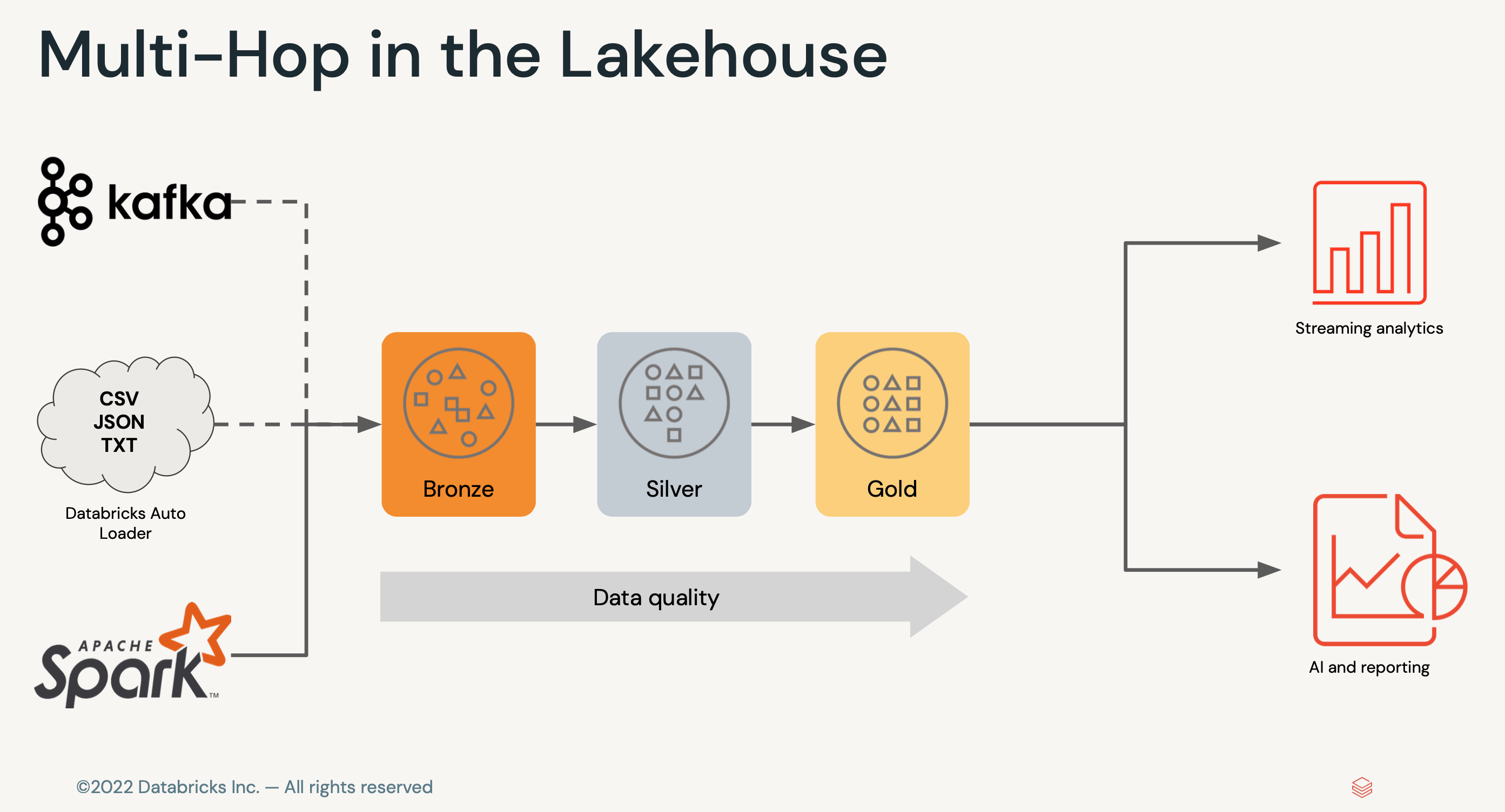
Bronze Layer (Raw Data)
- Typically just a raw copy of ingested data.
- Replaces traditional data lake.
- Provides efficient storage and querying of unprocessed history of data.
Silver Layer (Cleansed and Conformed Data)
- Reduces data storage complexity, latency, and redundancy.
- Optimizes ETL throughput and analytic query performance.
- Preserves grain of original data.
- Eliminates Duplicate records.
- Production schema is enforced.
- Data quality checks and corrupt data are quarantined.
Gold Layer (Curated Business-level tables)
- Powers ML applications, reporting, dashboards, and ad-hoc analytics.
- Refined views of data, typically with aggregations.
- Optimizes query performance for business-critical data.
Different Personas
- Data Engineer
- Data Analysts
- Data Scientists
[Avg. reading time: 0 minutes]
Data Engineering Model
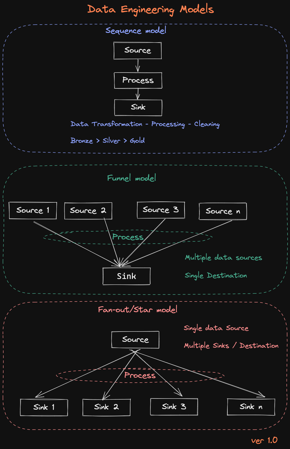
[Avg. reading time: 12 minutes]
Data Mesh
It’s a conceptual operational framework or platform architecture - not a tool or software.
It is built to address the complexities of managing data in large, distributed environments.
It shifts the traditional centralized approach of data management to a decentralized model.
The Data Mesh is a new approach based on a modern, distributed architecture for analytical data management.
The decentralized technique of data mesh distributes data ownership to domain-specific teams that manage, own, and serve the data as a product.
This concept is similar to Micro Service architecture.
The Monolithic Data Lake
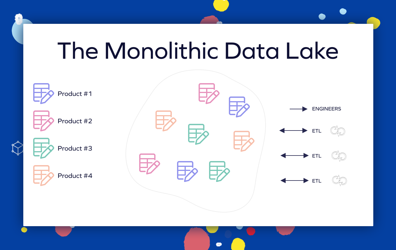
src: https://medium.com/yotpoengineering
There is no clear ownership and domain separation between the different assets. The ETL processes and engineer access to the platform are handled without a level of governance.
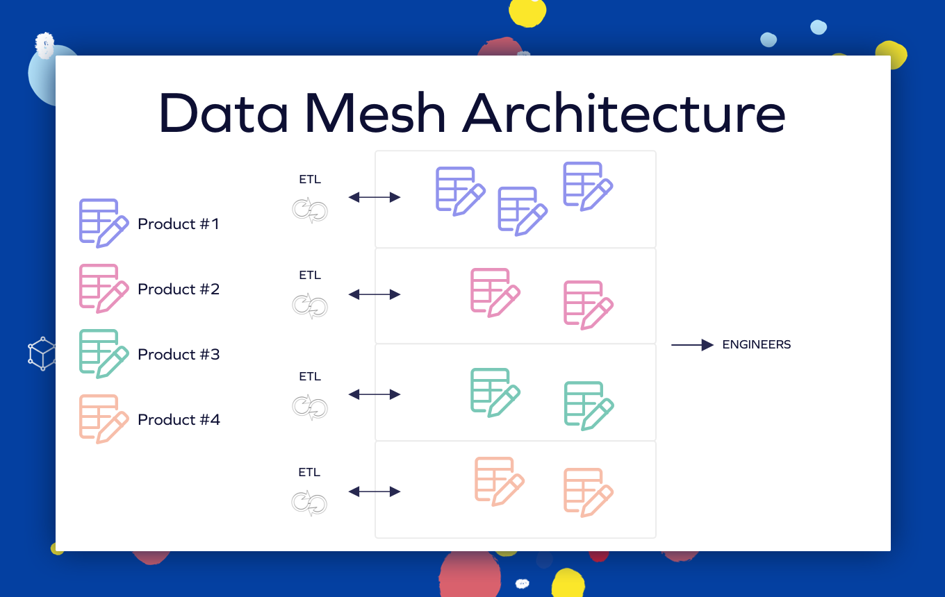 src: https://medium.com/yotpoengineering
There is a notable separation between different domains’ data sources and pipelines. The engineers are given a domain-agnostic interface to the data platform.
4 Pillars of Data Mesh (Core Principles)
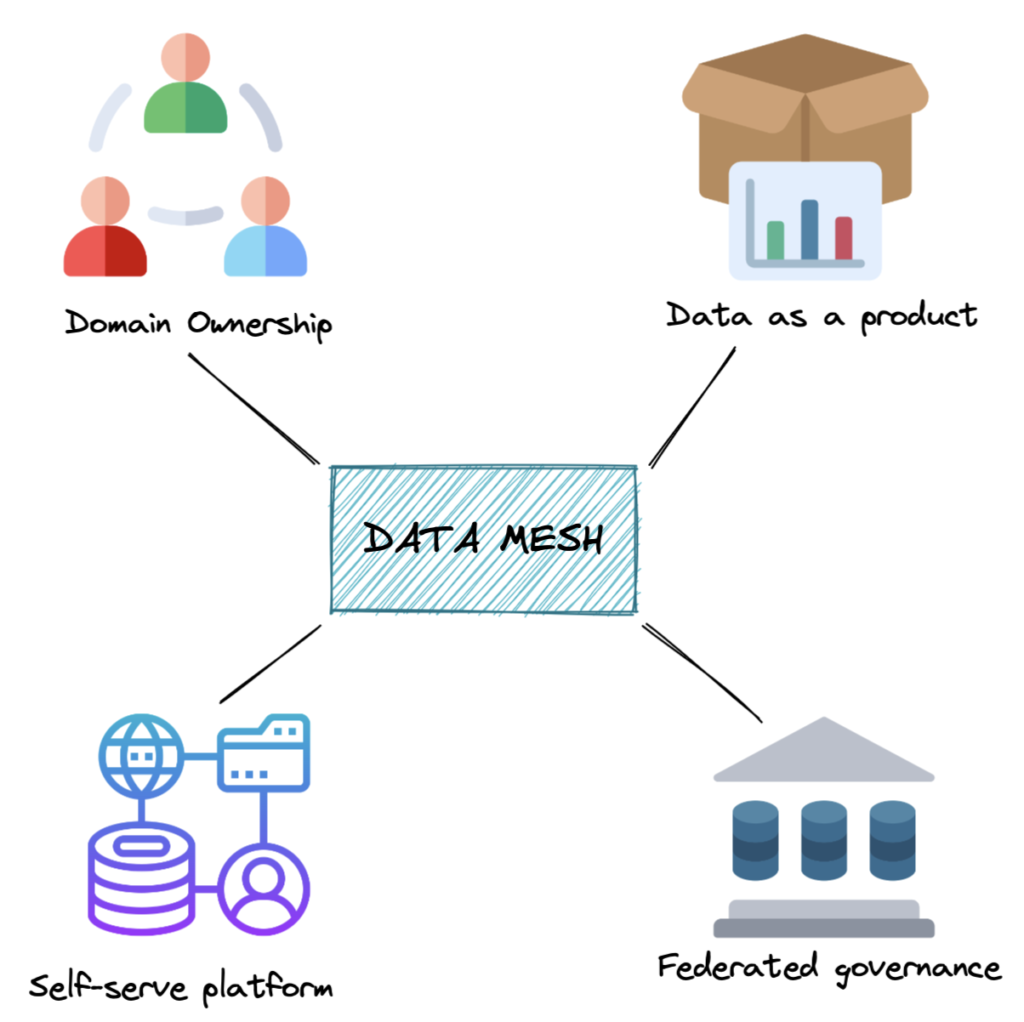 src: https://www.dremio.com/resources/guides/what-is-a-data-mesh/
Domain ownership: adopting a distributed architecture where domain teams - data producers - retain full responsibility for their data throughout its lifecycle, from capture through curation to analysis and reuse.
Data as a product: applying product management principles to the data analytics lifecycle, ensuring quality data is provided to data consumers who may be within and beyond the producer’s domain.
Self-service infrastructure platform: taking a domain-agnostic approach to the data analytics lifecycle, using standard tools and methods to build, run, and maintain interoperable data products.
Federated governance: Governance practices and policies are applied consistently across the organization, but implementation details are delegated to domain teams. This allows for scalability and adaptability, ensuring data remains trustworthy, secure, and compliant.
Data Products
Data products are an essential concept for data mesh. They are not meant to be datasets alone but data treated like a product:
They need to be
-
Discoverable
-
Trustworthy
-
Self-describing
-
Addressable and interoperable.
Besides data and metadata, they can contain code, dashboards, features, models, and other resources needed to create and maintain the data product.
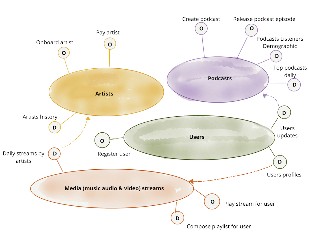 src: https://martinfowler.com/articles/data-mesh-principles.html
Benefits of Data Mesh in Data Management
Agility and Scalability - improving time-to-market and business domain agility.
Flexibility and independence - avoid becoming locked into one platform or data product.
Faster access to critical data - The self-serving model allows faster access.
Transparency for cross-functional use across teams - Due to decentralized data ownership, transparency is enabled.
Data Mesh Challenges
Cross-Domain Analytics - It is difficult to collaborate between different domain teams.
Consistent Data Standards - ensuring data products created by domain teams meet global standards.
Change in Data Management - Every team has autonomy over the data products they develop; managing them and balancing global and local standards can be tricky.
Skillsets: Success requires a blend of technical and product management skills within domain teams to manage data products effectively.
Technology Stack: Selecting and integrating the right technologies to support a self-serve data infrastructure can be challenging.
Slow to Adopt Process with Cost & Risk - The number of roles in each domain increases (data engineer, analyst, scientist, product owner). An org needs to establish well-defined roles and responsibilities to avoid causing MESS.
More reading
[Avg. reading time: 0 minutes]
Industry Trend
[Avg. reading time: 1 minute]
Roadmap - Data Engineer
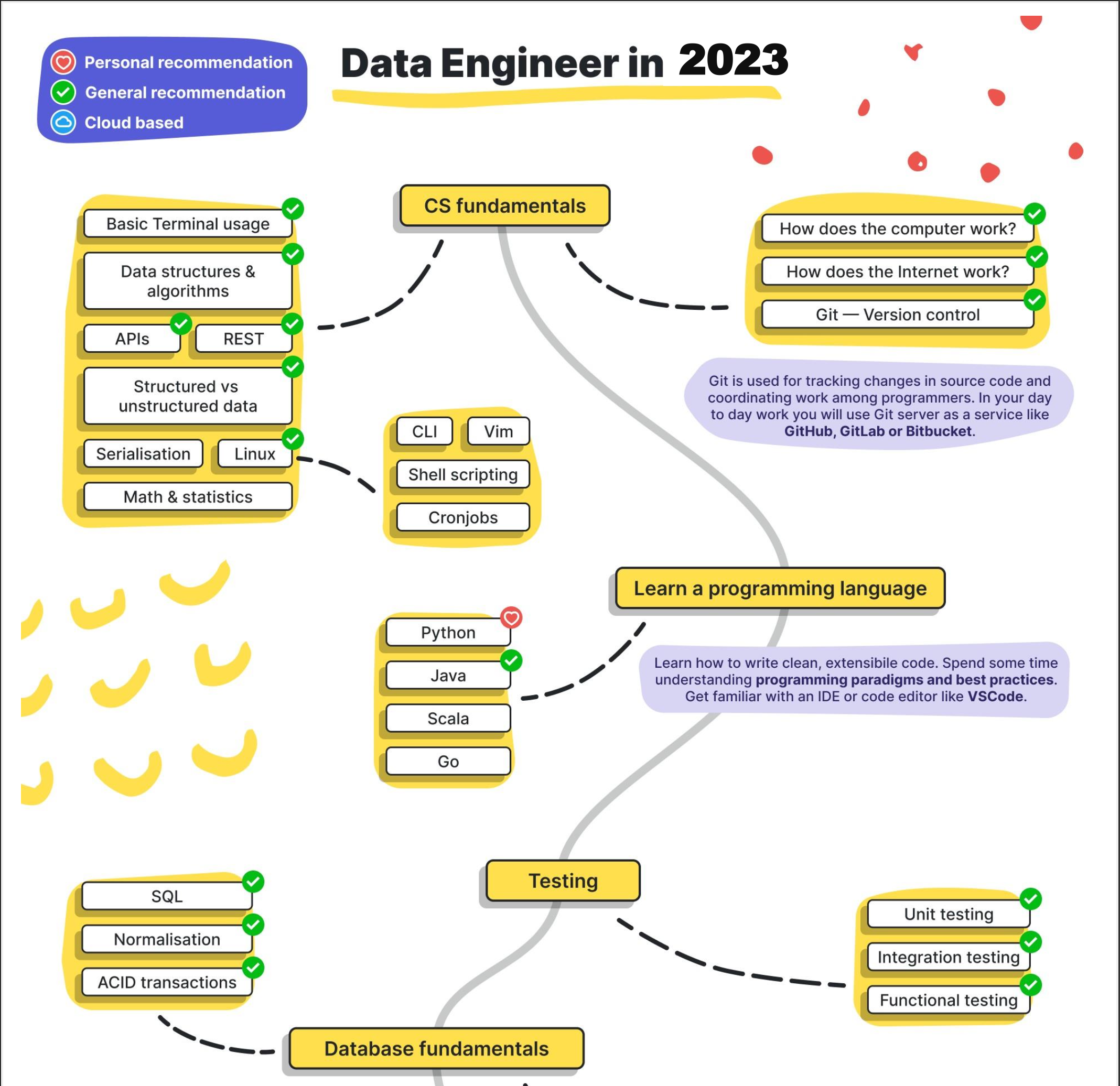
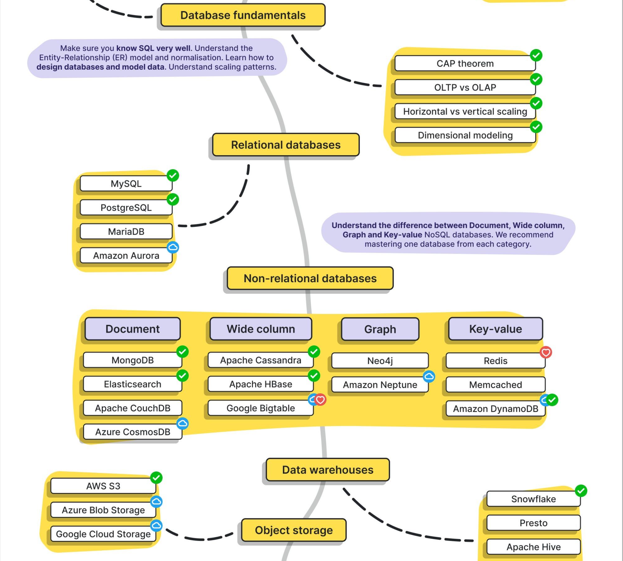
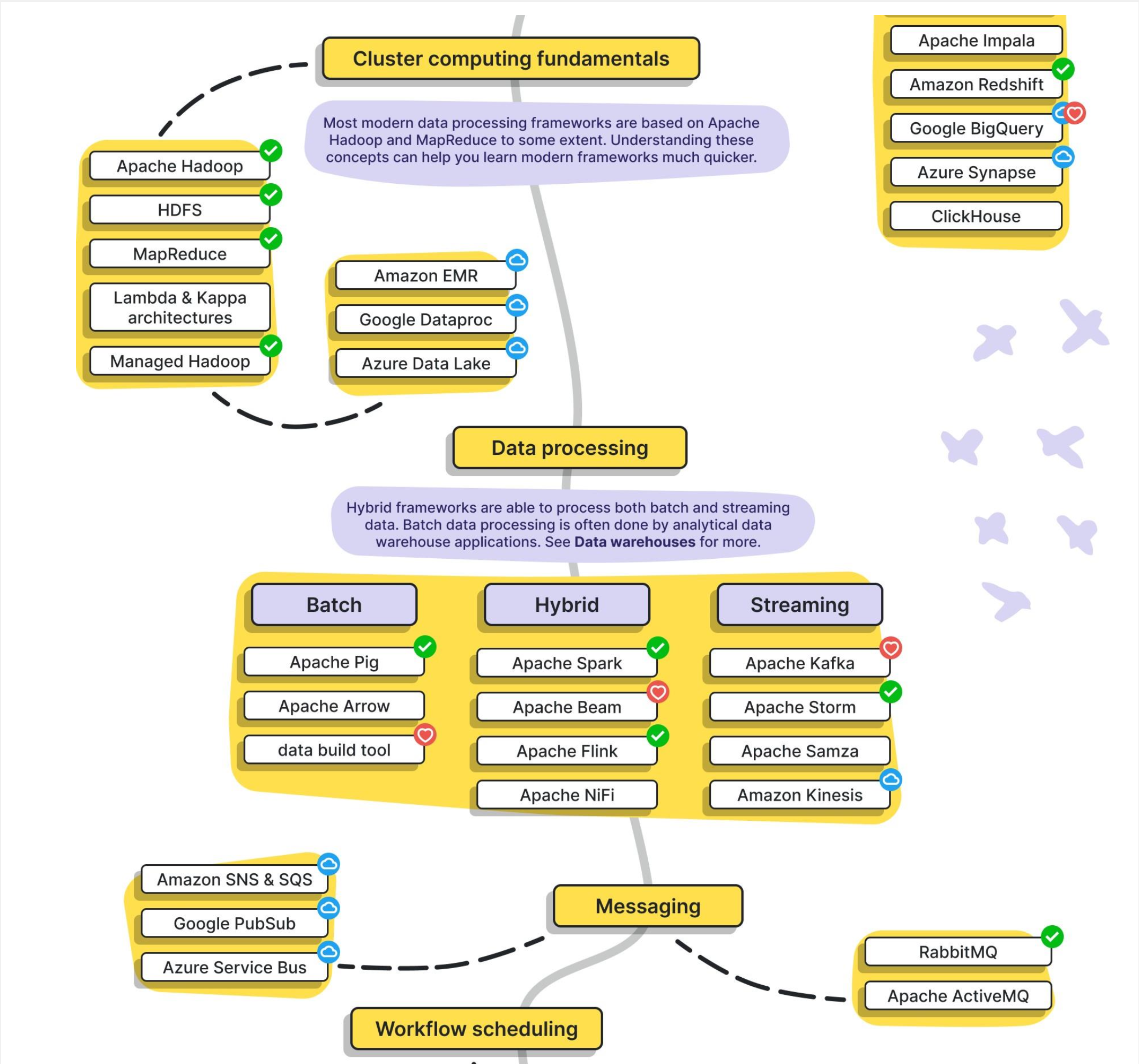

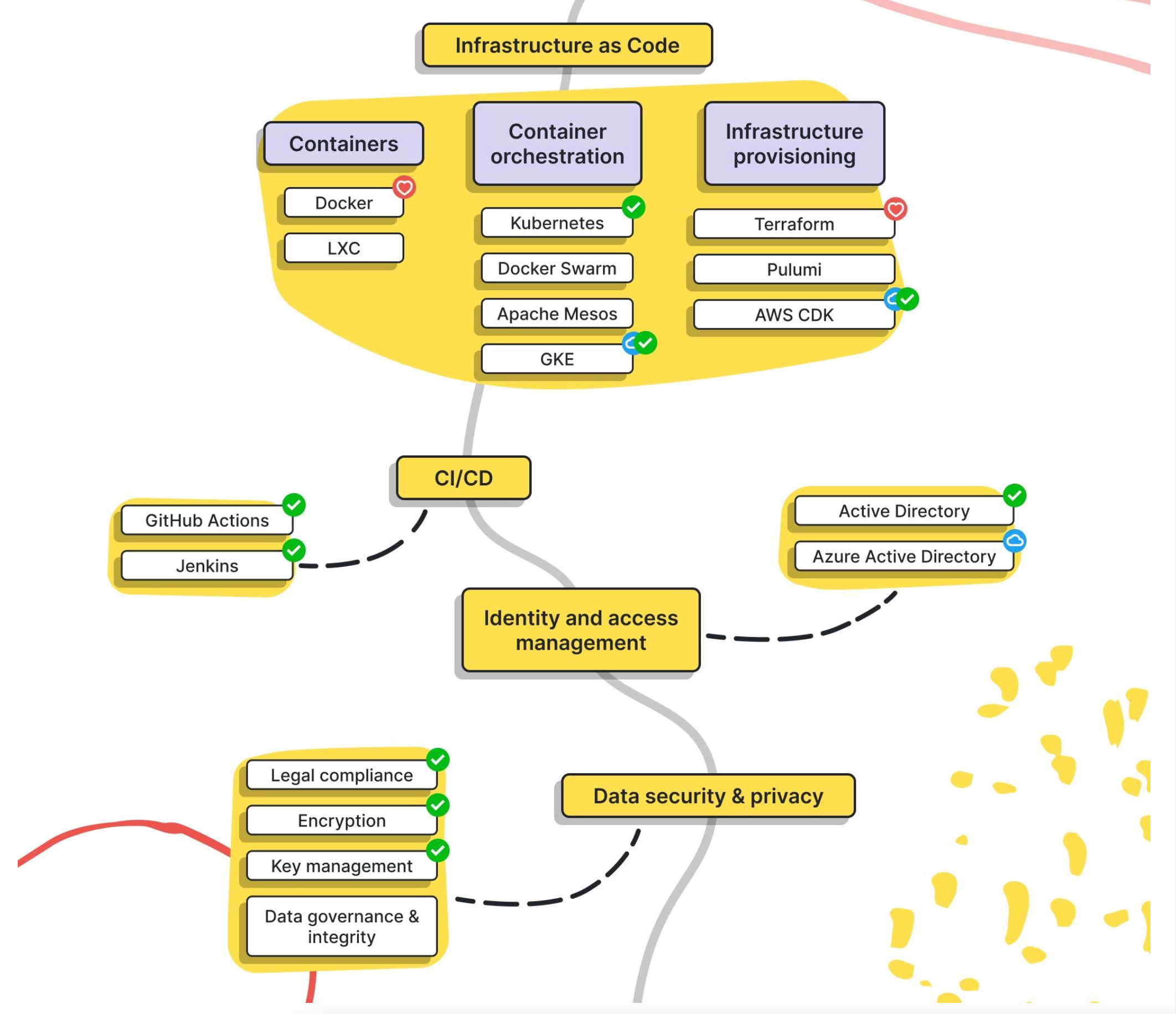
src: https://www.linkedin.com/in/pooja-jain-898253106/
[Avg. reading time: 4 minutes]
Notebooks vs IDE
| Feature | Notebooks (.ipynb) | Python Scripts (.py) |
|---|---|---|
| Use Case - DE | Quick prototyping, visualizing intermediate steps | Production-grade ETL, orchestration scripts |
| Use Case - DS | EDA, model training, visualization | Packaging models, deployment scripts |
| Interactivity | High – ideal for step-by-step execution | Low – executed as a whole |
| Visualization | Built-in (matplotlib, seaborn, plotly support) | Needs explicit code to save/show plots |
| Version Control | Harder to diff and merge | Easy to diff/merge in Git |
| Reusability | Lower, unless modularized | High – can be organized into functions, modules |
| Execution Context | Cell-based execution | Linear, top-to-bottom |
| Production Readiness | Poor (unless using tools like Papermill, nbconvert) | High – standard for CI/CD & Airflow etc. |
| Debugging | Easy with cell-wise changes | Needs breakpoints/logging |
| Integration | Jupyter, Colab, Databricks Notebooks | Any IDE (VSCode, PyCharm), scheduler integration |
| Documentation & Teaching | Markdown + code | Docstrings and comments only |
| Unit Tests | Not practical | Easily written using pytest, unittest |
| Package Management | Ad hoc, via %pip, %conda | Managed via requirements.txt, poetry, pipenv |
| Using Libraries | Easy for experimentation, auto-reloads supported | Cleaner imports, better for dependency resolution |
[Avg. reading time: 2 minutes]
Good Reads
Videos
ByteByteGo
It’s a very, very useful YT channel.
https://www.youtube.com/@ByteByteGo/videos
Loaded with lots and lots of useful information.
Career Path
Example: RoadMap for Python Learning
Cloud Providers
Run and Code Python in Cloud. Free and Affordable plans good for demonstration during Interviews.
Cheap/Affordable GPUs for AI Workloads
AI Tools

Tags
acid
/Data Format/Delta
acl
/NO SQL/Redis/Data Structures/Set
adbc
/Data Format/Arrow
adls
/Cloud Everywhere/Azure Cloud/Storages
aggregation
/NO SQL/Mongodb/Aggregation Pipeline
ai
/Big Data Overview/Trending Technologies
analysis
/Big Data Overview/How does it help?
aof
/NO SQL/Redis/Databases
/NO SQL/Redis/Persistence
api
/Advanced Python/Flask/API Testing
/Advanced Python/Flask/Flask Demo
/Advanced Python/Flask/Flask Demo-01
/Advanced Python/Flask/Flask Demo-02
/Advanced Python/Flask/Flask Demo-03
/Advanced Python/Flask/Flask Demo-04
/Advanced Python/Flask/Flask Demo-05
/Advanced Python/Flask/Setup
arrow
/Data Format/Arrow
/Data Format/Common Data Formats
authentication
/Advanced Python/Flask/Flask Demo-03
automation
/Developer Tools/JQ
availability
/Big Data Overview/Cap Theorem
avro
/Advanced Python/Serialization Deserialization
azure
/Cloud Everywhere/Azure Cloud
/Cloud Everywhere/Azure Cloud/Demo
/Cloud Everywhere/Azure Cloud/Services
/Cloud Everywhere/Azure Cloud/Storages
/Cloud Everywhere/Terraform
batch
/Data Engineering/Batch vs Streaming
bestpractices
/NO SQL/Mongodb/Mongodb Best Practices
bigdata
/Big Data Overview/Big Data Challenges
/Big Data Overview/Big Data Concerns
/Big Data Overview/Big Data Tools
/Big Data Overview/Eventual Consistency
/Big Data Overview/How does it help?
/Big Data Overview/Introduction
/Big Data Overview/Job Opportunities
/Big Data Overview/Learning Big Data means?
/Big Data Overview/Optimistic Concurrency
/Big Data Overview/The Big V's
/Big Data Overview/The Big V's/Other V's
/Big Data Overview/The Big V's/Variety
/Big Data Overview/The Big V's/Velocity
/Big Data Overview/The Big V's/Veracity
/Big Data Overview/The Big V's/Volume
/Big Data Overview/Trending Technologies
/Big Data Overview/What is Data?
/Data Format/Common Data Formats
/Data Format/Delta
/Data Format/JSON
/Data Format/Parquet
bigv
/Big Data Overview/The Big V's
/Big Data Overview/The Big V's/Variety
/Big Data Overview/The Big V's/Velocity
/Big Data Overview/The Big V's/Veracity
/Big Data Overview/The Big V's/Volume
binary
/Big Data Overview/The Big V's/Variety
cache
/NO SQL/Redis/Redis Cache Demo
calc
/Tools/CICD Tools
cap
/Big Data Overview/Cap Theorem
cd
/Tools/CICD Intro
/Tools/CICD Tools/CD Yaml
certification
/NO SQL/Mongodb/Further Reading
/NO SQL/Neo4J/Certification
challenges
/Cloud Everywhere/Challenges of Cloud Computing
chapter1
ci
/Tools/CICD Intro
cicd
/Tools/CICD Intro
/Tools/CICD Tools
classes
/Advanced Python/Python Classes
cli
/Cloud Everywhere/Azure Cloud/Demo
/Developer Tools/Duck DB
/Developer Tools/JQ
/NO SQL/Mongodb/Software
cloud
/Big Data Overview/Big Data Tools
/Cloud Everywhere/Challenges of Cloud Computing
columnar
/Big Data Overview/NO Sql Databases
/Data Format/Parquet
/NO SQL/Types of No SQL
commands
/NO SQL/Mongodb/Mongodb Commands
comprehension
/Advanced Python/Functional Programming Concepts
compressed
/Data Format/Parquet
concerns
/Big Data Overview/Big Data Concerns
concurrent
/Big Data Overview/Concurrent vs Parallel
consistency
/Big Data Overview/Cap Theorem
container
/Tools/Containers/Podman
/Tools/Containers/Podman Examples
/Tools/Containers/VMs or Containers
/Tools/Containers/What Container does
containers
/Cloud Everywhere/Azure Cloud/Storages
continuous
/Big Data Overview/Types of Data
crud
/Advanced Python/Flask/Flask Demo-02
csv
/Data Format/Common Data Formats
/NO SQL/Neo4J/Examples/Load CSV into Neo4J
dask
/Advanced Python/Data Frames
data
/Big Data Overview/What is Data?
data-profiling
/NO SQL/Neo4J/Examples/Data Profiling
database
/NO SQL/Redis/Databases
dataclass
/Advanced Python/Python Classes
dataformat
/Data Format/Arrow
/Data Format/Common Data Formats
/Data Format/JSON
/Data Format/Parquet
datalake
/Big Data Overview/Data Integration
dataquality
/Big Data Overview/Big Data Challenges
datatypes
/NO SQL/Mongodb/Data Types
decorator
/Advanced Python/Decorator
delta
/Data Format/Delta
demo
/NO SQL/Redis/Redis Cache Demo
deserialization
/Advanced Python/Serialization Deserialization
devops
/Cloud Everywhere/Terraform
discrete
/Big Data Overview/Types of Data
distributed
/Big Data Overview/Scaling
docker
/Tools/Containers/Podman
/Tools/Containers/Podman Examples
/Tools/Containers/VMs or Containers
dockerhub
/Tools/Containers/Podman Examples
docs
/Advanced Python/Code Quality & Safety
document
/NO SQL/Types of No SQL
documentation
/Advanced Python/Code Quality & Safety
documentdatabase
/NO SQL/Mongodb/Introduction
documentdb
/Big Data Overview/NO Sql Databases
domain
/Big Data Overview/DSL
dsl
/Big Data Overview/DSL
duckdb
/Developer Tools/Duck DB
elt
/Big Data Overview/Data Integration
errorhandling
/Advanced Python/Error Handling
ethics
/Big Data Overview/Big Data Challenges
etl
/Big Data Overview/Data Integration
eventhubs
/Data Engineering/Kafka/Different types of streaming
eventualconsistency
/Big Data Overview/Eventual Consistency
examples
/NO SQL/Redis/Data Structures/Redis Python
exception
/Advanced Python/Error Handling
faas
/Cloud Everywhere/Types of Cloud Services
flask
/Advanced Python/Flask/API Testing
/Advanced Python/Flask/Flask Demo
/Advanced Python/Flask/Flask Demo-01
/Advanced Python/Flask/Flask Demo-02
/Advanced Python/Flask/Flask Demo-03
/Advanced Python/Flask/Flask Demo-04
/Advanced Python/Flask/Flask Demo-05
/Advanced Python/Flask/Setup
flightrpc
/Data Format/Arrow
flightsql
/Data Format/Arrow
flushall
/NO SQL/Redis/Databases
flushdb
/NO SQL/Redis/Databases
functional
/Advanced Python/Functional Programming Concepts
functions
/NO SQL/Neo4J/Examples/Commonly Used Functions
funtask
/NO SQL/Mongodb/Fun Task
generator
/Advanced Python/Functional Programming Concepts
geospatial
/NO SQL/Redis/Data Structures/Geospatial Index
git
/Advanced Python/Flask/Flask Demo
/Advanced Python/Flask/Flask Demo-01
/Advanced Python/Flask/Flask Demo-02
/Advanced Python/Flask/Flask Demo-03
/Advanced Python/Flask/Flask Demo-04
/Advanced Python/Flask/Flask Demo-05
github
/Tools/CICD Tools/CI Yaml
githubactions
/Tools/CICD Tools
/Tools/CICD Tools/CI Yaml
gpl
/Big Data Overview/GPL
graph
/NO SQL/Types of No SQL
graphdatabase
/NO SQL/Neo4J
graphdb
/Big Data Overview/NO Sql Databases
ha
/Cloud Everywhere/High Availability
hash
/NO SQL/Redis/Data Structures/Hash
hello-world
/NO SQL/Neo4J/Hello World
hierarchical
/Data Format/JSON
highavailability
/Cloud Everywhere/High Availability
horizontal
/Big Data Overview/Scaling
html
/Big Data Overview/DSL
iaas
/Cloud Everywhere/Types of Cloud Services
image
/Big Data Overview/The Big V's/Variety
import
/NO SQL/Mongodb/Import
info
/Advanced Python/Logging
insert
/NO SQL/Mongodb/Insert Document
interoperability
/Big Data Overview/Big Data Challenges
introduction
/NO SQL/Mongodb/Introduction
iot
/Big Data Overview/Trending Technologies
jobs
/Big Data Overview/Job Opportunities
jq
/Developer Tools/JQ
json
/Big Data Overview/The Big V's/Variety
/Data Format/JSON
/Developer Tools/JQ
/NO SQL/Mongodb/Import
/NO SQL/Mongodb/Sample JSON
/NO SQL/Redis/Redis JSON
jwt
/Advanced Python/Flask/Flask Demo-04
kafka
/Big Data Overview/Big Data Tools
/Data Engineering/Kafka
/Data Engineering/Kafka/Kafka Software
/Data Engineering/Kafka/Kafka use cases
/Data Engineering/Kafka/Python Scripts
keyvalue
/Big Data Overview/NO Sql Databases
/NO SQL/Redis
/NO SQL/Types of No SQL
keywords
/NO SQL/Redis/Terms to know
kinesis
/Data Engineering/Kafka/Different types of streaming
/Data Engineering/Kafka/Kafka Software
knowledge
/Big Data Overview/How does it help?
lambda
/Advanced Python/Functional Programming Concepts
learning
/Big Data Overview/Learning Big Data means?
/Big Data Overview/Learning Big Data means?
lint
/Developer Tools/Other Python Tools
/Developer Tools/Poetry
list
/NO SQL/Redis/Data Structures/List
logging
/Advanced Python/Logging
logicaloperators
/NO SQL/Mongodb/Logical Operators
lpush
/NO SQL/Redis/Data Structures/List
memoization
/Advanced Python/Decorator
message
/NO SQL/Redis/Data Structures/Pub Sub
mitigation
/Big Data Overview/Big Data Concerns
mongodb
/NO SQL/Mongodb/Aggregation Pipeline
/NO SQL/Mongodb/Data Types
/NO SQL/Mongodb/Fun Task
/NO SQL/Mongodb/Fun Task/Sample
/NO SQL/Mongodb/Further Reading
/NO SQL/Mongodb/Import
/NO SQL/Mongodb/Insert Document
/NO SQL/Mongodb/Introduction
/NO SQL/Mongodb/Logical Operators
/NO SQL/Mongodb/Mongodb Best Practices
/NO SQL/Mongodb/Mongodb Commands
/NO SQL/Mongodb/Operators
/NO SQL/Mongodb/Querying Mongodb
/NO SQL/Mongodb/Sample JSON
/NO SQL/Mongodb/Software
/NO SQL/Mongodb/Update & Remove
mypy
/Developer Tools/Other Python Tools
/Developer Tools/Poetry
mysql
/Advanced Python/Flask/Flask Demo-05
/NO SQL/Neo4J/Examples/Mysql Neo4j
/NO SQL/Redis/Redis - (Rdbms) Mysql
/NO SQL/Redis/Redis Cache Demo
mysqlcloud
/Advanced Python/Flask/Setup
namespaces
/NO SQL/Redis/Data Structures/Strings
neo4j
/NO SQL/Neo4J
/NO SQL/Neo4J/Certification
/NO SQL/Neo4J/Examples/Commonly Used Functions
/NO SQL/Neo4J/Examples/Create Nodes
/NO SQL/Neo4J/Examples/Data Profiling
/NO SQL/Neo4J/Examples/Load CSV into Neo4J
/NO SQL/Neo4J/Examples/Mysql Neo4j
/NO SQL/Neo4J/Examples/Putting it all-together
/NO SQL/Neo4J/Examples/Python Scripts
/NO SQL/Neo4J/Examples/Queries
/NO SQL/Neo4J/Examples/Relation
/NO SQL/Neo4J/Examples/Sample
/NO SQL/Neo4J/Examples/Sample Transactions
/NO SQL/Neo4J/Examples/Update Nodes
/NO SQL/Neo4J/Hello World
/NO SQL/Neo4J/Neo4j Components
/NO SQL/Neo4J/Neo4j Terms
/NO SQL/Neo4J/Software
neo4j-components
/NO SQL/Neo4J/Neo4j Components
neo4j-terms
/NO SQL/Neo4J/Neo4j Terms
nodes
/NO SQL/Neo4J/Examples/Create Nodes
nominal
/Big Data Overview/Types of Data
nosql
/Big Data Overview/NO Sql Databases
/NO SQL/Redis/Data Structures/List
/NO SQL/Redis/Data Structures/Set
/NO SQL/Redis/Data Structures/Strings
/NO SQL/Redis/Persistence
/NO SQL/Redis/Redis JSON
/NO SQL/Redis/Redis Search
/NO SQL/Redis/Timeseries
/NO SQL/Types of No SQL
opensource
/NO SQL/Types of No SQL
operators
/NO SQL/Mongodb/Operators
optimistic
/Big Data Overview/Optimistic Concurrency
ordinal
/Big Data Overview/Types of Data
otherv
/Big Data Overview/The Big V's/Other V's
overview
/Big Data Overview/Introduction
paas
/Cloud Everywhere/Types of Cloud Services
pandas
/Advanced Python/Data Frames
parallelprogramming
/Big Data Overview/Concurrent vs Parallel
parquet
/Data Format/Common Data Formats
/Data Format/Parquet
/Developer Tools/Duck DB
parser
/Developer Tools/JQ
partitiontolerant
/Big Data Overview/Cap Theorem
pep
/Developer Tools/Other Python Tools
persistence
/NO SQL/Redis/Persistence
pipeline
/Big Data Overview/Data Integration
podman
/Tools/Containers/Podman
/Tools/Containers/Podman Examples
poetry
/Developer Tools/Poetry
polars
/Advanced Python/Data Frames
privacy
/Big Data Overview/Big Data Challenges
pubsub
/Data Engineering/Batch vs Streaming
/Data Engineering/Kafka/Kafka Software
/NO SQL/Redis/Data Structures/Pub Sub
pytest
/Advanced Python/Flask/Flask Demo Testing
/Advanced Python/Unit Testing
python
/Advanced Python/Flask/Flask Demo
/Advanced Python/Flask/Flask Demo-01
/Advanced Python/Flask/Flask Demo-02
/Advanced Python/Flask/Flask Demo-03
/Advanced Python/Flask/Flask Demo-04
/Advanced Python/Flask/Flask Demo-05
/Big Data Overview/GPL
/Data Engineering/Kafka/Python Scripts
/Developer Tools/Poetry
/NO SQL/Redis/Data Structures/Redis Python
pythonscripts
/NO SQL/Neo4J/Examples/Python Scripts
qualitative
/Big Data Overview/Types of Data
quantitative
/Big Data Overview/Types of Data
queries
/NO SQL/Neo4J/Examples/Putting it all-together
/NO SQL/Neo4J/Examples/Queries
query
/NO SQL/Mongodb/Querying Mongodb
rawdata
/Big Data Overview/Data Integration
/Big Data Overview/How does it help?
rdb
/NO SQL/Redis/Databases
/NO SQL/Redis/Persistence
rdbms
realtime
/Big Data Overview/Big Data Challenges
/Data Engineering/Kafka
redis
/NO SQL/Redis
/NO SQL/Redis/Data Structures/Geospatial Index
/NO SQL/Redis/Data Structures/List
/NO SQL/Redis/Data Structures/Set
/NO SQL/Redis/Data Structures/Strings
/NO SQL/Redis/Persistence
/NO SQL/Redis/Redis - (Rdbms) Mysql
/NO SQL/Redis/Redis JSON
/NO SQL/Redis/Redis Search
/NO SQL/Redis/Terms to know
/NO SQL/Redis/Timeseries
/NO SQL/Redis/Use Cases
redis_python
/NO SQL/Redis/Data Structures/Redis Python
redisgraph
/NO SQL/Redis/Terms to know
redisshard
/NO SQL/Redis/Terms to know
relation
/NO SQL/Neo4J/Examples/Relation
remove
/NO SQL/Mongodb/Update & Remove
robotics
/Big Data Overview/Trending Technologies
rpush
/NO SQL/Redis/Data Structures/List
ruff
/Developer Tools/Other Python Tools
/Developer Tools/Poetry
rust
/Big Data Overview/GPL
/Developer Tools/UV
saas
/Cloud Everywhere/Types of Cloud Services
sadd
/NO SQL/Redis/Data Structures/Set
salesdata
/NO SQL/Neo4J/Examples/Load CSV into Neo4J
sample
/NO SQL/Neo4J/Examples/Sample
samplejson
/NO SQL/Mongodb/Sample JSON
scaling
/Big Data Overview/Scaling
search
/NO SQL/Redis/Redis Search
semistructured
/Big Data Overview/The Big V's/Variety
serialization
/Advanced Python/Serialization Deserialization
services
/Cloud Everywhere/Azure Cloud/Services
singlefiledatabase
/Developer Tools/Duck DB
smembers
/NO SQL/Redis/Data Structures/Set
software
/NO SQL/Mongodb/Software
/NO SQL/Neo4J/Software
softwares
/Data Engineering/Kafka/Kafka Software
spark
/Big Data Overview/Big Data Tools
sql
/Big Data Overview/DSL
stateful
/Data Engineering/Kafka/Different types of streaming
stateless
/Data Engineering/Kafka/Different types of streaming
storage
/Big Data Overview/Big Data Challenges
storageaccount
/Cloud Everywhere/Azure Cloud/Storages
streaming
/Data Engineering/Batch vs Streaming
strings
/NO SQL/Redis/Data Structures/Strings
structured
/Big Data Overview/The Big V's/Variety
studio3t
/NO SQL/Mongodb/Software
technologies
/Big Data Overview/Trending Technologies
terraform
/Cloud Everywhere/Terraform
test
/Advanced Python/Flask/Flask Demo Testing
testing
/Advanced Python/Flask/API Testing
timeseries
/NO SQL/Redis/Timeseries
tools
/Big Data Overview/Big Data Tools
/Developer Tools/Duck DB
/Developer Tools/JQ
traditionaldata
/Big Data Overview/What is Data?
transaction
/NO SQL/Neo4J/Examples/Sample Transactions
try
/Advanced Python/Error Handling
tsdb
/NO SQL/Redis/Timeseries
twitter
/NO SQL/Mongodb/Fun Task/Sample
unittest
/Advanced Python/Flask/Flask Demo Testing
unittesting
/Advanced Python/Unit Testing
unstructured
/Big Data Overview/The Big V's/Variety
update
/NO SQL/Mongodb/Update & Remove
/NO SQL/Neo4J/Examples/Update Nodes
upstash
/Advanced Python/Flask/Setup
usecases
/Data Engineering/Kafka/Kafka use cases
/NO SQL/Redis/Use Cases
uv
/Developer Tools/UV
validity
/Big Data Overview/The Big V's/Other V's
value
/Big Data Overview/The Big V's/Other V's
velocity
/Big Data Overview/The Big V's/Velocity
venv
/Developer Tools/UV
veracity
/Big Data Overview/The Big V's/Veracity
version
/Big Data Overview/The Big V's/Other V's
vertical
/Big Data Overview/Scaling
vm
/Tools/Containers/VMs or Containers
volume
/Big Data Overview/The Big V's/Volume
webapp
/NO SQL/Redis/Redis - (Rdbms) Mysql
worksforme
/Tools/Containers/What Container does
xml
/Big Data Overview/The Big V's/Variety
yaml
/Tools/CICD Tools/CD Yaml
/Tools/CICD Tools/CI Yaml